Subgradients and Online-to-Batch conversion

This post is part of the lecture notes of my class “Introduction to Online Learning” at Boston University, Fall 2019. I will publish two lectures per week.

You can find the lectures I published till now here.

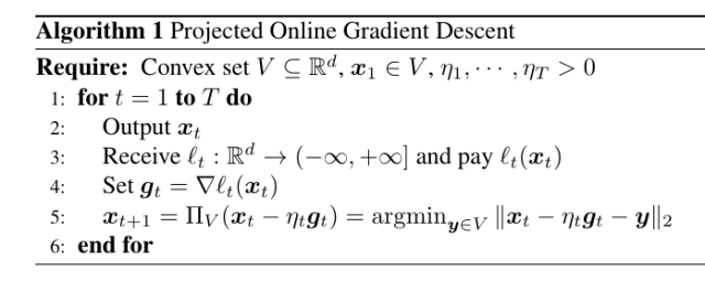
Last time, we introduced Projected Online Gradient Descent:

pogd

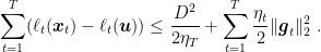
And we proved the following regret guarantee:

Theorem 1 Let ${V\subseteq {\mathbb R}^d}$ a closed non-empty convex set with diameter ${D}$ , i.e. ${\max_{{\boldsymbol x},{\boldsymbol y}\in V} \|{\boldsymbol x}-{\boldsymbol y}\|_2 \leq D}$ . Let ${\ell_1, \cdots, \ell_T}$ an arbitrary sequence of convex functions ${\ell_t:{\mathbb R}^d \rightarrow (-\infty, +\infty]}$ differentiable in open sets containing ${V}$ for ${t=1, \dots,T}$ . Pick any ${{\boldsymbol x}_1 \in V}$ assume ${\eta_{t+1}\leq \eta_{t}, \ t=1, \dots, T}$ . Then, ${\forall {\boldsymbol u} \in V}$ , the following regret bound holds

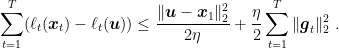
$\displaystyle \sum_{t=1}^T (\ell_t({\boldsymbol x}_t) - \ell_t({\boldsymbol u})) \leq \frac{D^2}{2\eta_{T}} + \sum_{t=1}^T \frac{\eta_t}{2} \|{\boldsymbol g}_t\|^2_2~.$

Moreover, if ${\eta_t}$ is constant, i.e. ${\eta_t=\eta \ \forall t=1,\cdots,T}$ , we have

$\displaystyle \sum_{t=1}^T (\ell_t({\boldsymbol x}_t) - \ell_t({\boldsymbol u})) \leq \frac{\|{\boldsymbol u}-{\boldsymbol x}_1\|_2^2}{2\eta} + \frac{\eta}{2} \sum_{t=1}^T \|{\boldsymbol g}_t\|^2_2~.$

However, the differentiability assumption for the ${\ell_t}$ is quite strong. What happens when the losses are convex but not differentiable? For example ${\ell_t(x)=|x-10|}$ . Note that this situation is more common than one would think. For example, the hinge loss, ${f({\boldsymbol w})=\max(1-y\langle {\boldsymbol w},{\boldsymbol x}\rangle,0)}$ , and the ReLU activation function used in neural networks, ${f(x)=\max(x,0)}$ , are not differentiable. It turns out that we can just use Online Gradient Descent, substituting the subgradients to the gradients. For this, we need some more convex analysis!

1. Convex Analysis Bits: Subgradients

First, we need a technical definition.

Definition 2 If a function ${f}$ is nowhere ${-\infty}$ and finite somewhere, then ${f}$ is called proper.

In these class, we are mainly interested in convex proper functions, that basically better conform to our intuition of what a convex function looks like.

Let’s first define formally what is a subgradient.

Definition 3 For a proper function ${f:{\mathbb R}^d \rightarrow (-\infty, +\infty]}$ , we define a subgradient of ${f}$ in ${{\boldsymbol x} \in {\mathbb R}^d}$ as a vector ${{\boldsymbol g} \in {\mathbb R}^d}$ that satisfies

$\displaystyle f({\boldsymbol y})\geq f({\boldsymbol x}) + \langle {\boldsymbol g}, {\boldsymbol y}-{\boldsymbol x}\rangle, \ \forall {\boldsymbol y} \in {\mathbb R}^d~.$

Basically, a subgradient of ${f}$ in ${{\boldsymbol x}}$ is any vector ${{\boldsymbol g}}$ that allows us to construct a linear lower bound to ${f}$ . Note that the subgradient is not unique, so we denote the set of subgradients of ${f}$ in ${{\boldsymbol x}}$ by ${\partial f({\boldsymbol x})}$ , called subdifferential of ${f}$ at ${{\boldsymbol x}}$ .

Observe that if ${f}$ is proper and convex, then ${\partial f({\boldsymbol x})}$ is empty for ${{\boldsymbol x} \notin \mathop{\mathrm{dom}} f}$ , because the inequality cannot be satisfied when ${f({\boldsymbol x})=+\infty}$ . Also, the domain of ${\partial f}$ , denoted by ${\mathop{\mathrm{dom}} \partial f}$ , is the set of all ${{\boldsymbol x} \in {\mathbb R}^d}$ such that ${\partial f(x)}$ is nonempty; it is a subset of ${\mathop{\mathrm{dom}} f}$ . A proper convex function ${f}$ is always subdifferentiable in ${\mathop{\mathrm{int}} \mathop{\mathrm{dom}} f}$ (Rockafellar, R. T., 1970, Theorem 23.4). If the function is convex, differentiable in ${{\boldsymbol x}}$ , and ${f}$ is finite in ${{\boldsymbol x}}$ , we have that the subdifferential is composed by a unique element equal to ${\nabla f({\boldsymbol x})}$ (Rockafellar, R. T., 1970, Theorem 25.1).

Also, we can also calculate the subgradient of sum of functions.

Theorem 4 (Rockafellar, R. T., 1970, Theorem 23.8,Bauschke, H. H. and Combettes, P. L., 2011, Corollary 16.39) Let ${f_1,\ldots ,f_m}$ be proper convex functions on ${{\mathbb R}^d}$ , and ${f=f_1+\cdots+f_m}$ . Then ${\partial f({\boldsymbol x}) \supset \partial f_1({\boldsymbol x}) + \cdots + \partial f_m({\boldsymbol x}), \forall {\boldsymbol x}}$ . If ${\mathop{\mathrm{dom}} f_m \cap \bigcap_{i=1}^{m-1} \mathop{\mathrm{int}} \mathop{\mathrm{dom}} f_i \neq \{\}}$ , then actually ${\partial f({\boldsymbol x}) = \partial f_1({\boldsymbol x}) + \cdots + \partial f_m({\boldsymbol x}), \forall x}$ .

Example 1 Let ${f(x)=|x|}$ , then the subdifferential set ${\partial f(x)}$ is

$\displaystyle \partial f(x) = \begin{cases} \{1\}, & x>0,\\ [-1,1], & x=0\\ \{-1\}, & x<0~. \end{cases}$

Example 2 Let’s calculate the subgradient of the indicator function for a non-empty convex set ${V \subset {\mathbb R}^d}$ . By definition, ${{\boldsymbol g} \in \partial i_V({\boldsymbol x})}$ if

$\displaystyle i_V({\boldsymbol y}) \geq i_V({\boldsymbol x}) + \langle {\boldsymbol g}, {\boldsymbol y}-{\boldsymbol x}\rangle, \ \forall {\boldsymbol y} \in {\mathbb R}^d~.$

This condition implies that ${{\boldsymbol x} \in V}$ and ${0 \geq \langle {\boldsymbol g}, {\boldsymbol y}-{\boldsymbol x}\rangle, \forall {\boldsymbol y} \in V}$ (because for ${{\boldsymbol y} \notin V}$ the inequality is always verified). The set of all ${{\boldsymbol g}}$ that satisfies the above inequality is called the normal cone of ${V}$ at ${{\boldsymbol x}}$ . Note that the normal cone for any ${{\boldsymbol x}\in \mathop{\mathrm{int}} V = \{\boldsymbol{0}\}}$ (Hint: take ${{\boldsymbol y}={\boldsymbol x}+\epsilon{\boldsymbol g}}$ ). For example, for ${V=\{{\boldsymbol x} \in {\mathbb R}^d| \|{\boldsymbol x}\|_2\leq 1\}}$ , ${\partial i_V({\boldsymbol x}) = \{\alpha {\boldsymbol x}|\alpha \geq0\}}$ for all ${{\boldsymbol x} : \|{\boldsymbol x}\|=1}$ .

Another useful theorem is to calculate the subdifferential of the pointwise maximum of convex functions.

Theorem 5 (Bauschke, H. H. and Combettes, P. L., 2011, Theorem 18.5) Let ${(f_i)_{i\in I}}$ be a finite set of convex functions from ${{\mathbb R}^d}$ to ${(-\infty, +\infty]}$ and suppose ${{\boldsymbol x} \in \bigcap_{i \in I} \mathop{\mathrm{dom}} f_i}$ and ${f_i}$ continuous at ${{\boldsymbol x}}$ . Set ${F = \max_{i \in I} f_i}$ and let ${A({\boldsymbol x}) = \{i \in I | f_i({\boldsymbol x})=F({\boldsymbol x})\}}$ the set of the active functions. Then

$\displaystyle \partial F({\boldsymbol x}) = \mathop{\mathrm{conv}} \bigcup_{i \in A({\boldsymbol x})} \partial f_i({\boldsymbol x})~.$

Example 3 (Subgradients of the Hinge loss) Consider the loss ${\ell({\boldsymbol x})=\max(1-\langle {\boldsymbol z},{\boldsymbol x}\rangle,0)}$ for ${{\boldsymbol z} \in {\mathbb R}^d}$ . The subdifferential set if

$\displaystyle \partial \ell({\boldsymbol x}) = \begin{cases} \{\boldsymbol{0}\}, & 1-\langle {\boldsymbol z},{\boldsymbol x}\rangle <0\\ \{-\alpha {\boldsymbol z}| \alpha \in [0,1]\}, & 1-\langle {\boldsymbol z},{\boldsymbol x}\rangle =0\\ \{-{\boldsymbol z}\}, & \text{otherwise} \end{cases}~.$

Definition 6 Let ${f:{\mathbb R}^d \rightarrow (-\infty, +\infty]}$ is ${L}$ -Lipschitz over a set ${V}$ w.r.t a norm ${\|\cdot\|}$ if ${|f({\boldsymbol x})-f({\boldsymbol y})|\leq L \|{\boldsymbol x}-{\boldsymbol y}\|, \ \forall {\boldsymbol x},{\boldsymbol y} \in V}$ .

We also have this handy result that upper bounds the norm of subgradients of convex Lipschitz functions.

Theorem 7 Let ${f:{\mathbb R}^d \rightarrow (-\infty, +\infty]}$ proper and convex. Then, ${f}$ is ${L}$ -Lipschitz in ${\mathop{\mathrm{int}} \mathop{\mathrm{dom}} f}$ w.r.t. the L2 norm iff for all ${{\boldsymbol x} \mathop{\mathrm{int}} \mathop{\mathrm{dom}} f}$ and ${{\boldsymbol g} \in \partial f({\boldsymbol x})}$ we have ${\|{\boldsymbol g}\|_2\leq L}$ .

Proof: Assume ${f}$ ${L}$ -Lipschitz, then ${|f({\boldsymbol x})-f({\boldsymbol y})|\leq L \|{\boldsymbol x}-{\boldsymbol y}\|_2, \ \forall {\boldsymbol x}, {\boldsymbol y} \in \mathop{\mathrm{dom}} f}$ . For ${\epsilon>0}$ small enough ${{\boldsymbol y}={\boldsymbol x}+\epsilon \frac{{\boldsymbol g}}{\|{\boldsymbol g}\|_2} \in \mathop{\mathrm{int}} \mathop{\mathrm{dom}} f}$ , then

$\displaystyle \begin{aligned} L \epsilon = L \|{\boldsymbol x}-{\boldsymbol y}\|_2 \geq |f({\boldsymbol y})-f({\boldsymbol x})| \geq f({\boldsymbol y}) - f({\boldsymbol x}) \geq \langle {\boldsymbol g}, {\boldsymbol y} -{\boldsymbol x}\rangle = \epsilon \|{\boldsymbol g}\|_2, \end{aligned}$

that implies that ${\|{\boldsymbol g}\|_2\leq L}$ .

For the other implication, the definition of subgradient and Cauchy-Schwartz inequalities gives us

$\displaystyle f({\boldsymbol x})-f({\boldsymbol y}) \leq \|{\boldsymbol g}\|_2 \|{\boldsymbol x}-{\boldsymbol y}\|_2 \leq L \|{\boldsymbol x}-{\boldsymbol y}\|_2,$

for any ${{\boldsymbol x},{\boldsymbol y} \in \mathop{\mathrm{int}} \mathop{\mathrm{dom}} f}$ . Taking ${{\boldsymbol g} \in \partial f({\boldsymbol y})}$ , we also get

$\displaystyle f({\boldsymbol y})-f({\boldsymbol x}) \leq L \|{\boldsymbol x}-{\boldsymbol y}\|_2,$

that completes the proof. $\Box$

2. Analysis with Subgradients

As I promised you, with the proper mathematical tools, the analyzing online algorithms becomes easy. Indeed, switching from gradient to subgradient comes for free! In fact, our analysis of OGD with differentiable losses holds as is using subgradients instead of gradients. The reason is that the only property of the gradients that we used in our proof was that

$\displaystyle \ell_t({\boldsymbol x}) - \ell_t({\boldsymbol u}) \leq \langle {\boldsymbol g}_t, {\boldsymbol x}_t - {\boldsymbol u}\rangle,$

where ${{\boldsymbol g}_t = \nabla \ell_t({\boldsymbol x}_t)}$ . However, the exact same property holds when ${{\boldsymbol g}_t \in \partial \ell_t({\boldsymbol x}_t)}$ . So, we can state the Online Subgradient descent algorithm in the following way, where the only difference is line 4.

posd

Also, the regret bounds we proved holds as well, just changing differentiability with subdifferentiability and gradients with subgradients.

3. From Convex Losses to Linear Losses

Let’s take a deeper look at this step

$\displaystyle \ell_t({\boldsymbol x}_t) - \ell_t({\boldsymbol u}) \leq \langle {\boldsymbol g}_t, {\boldsymbol x}_t-{\boldsymbol u}\rangle, \forall {\boldsymbol u} \in {\mathbb R}^d~.$

And summing over time, we have

$\displaystyle \sum_{t=1}^T \ell_t({\boldsymbol x}_t) - \ell_t({\boldsymbol u}) \leq \sum_{t=1}^T \langle {\boldsymbol g}_t, {\boldsymbol x}_t-{\boldsymbol u}\rangle, \forall {\boldsymbol u} \in {\mathbb R}^d~.$

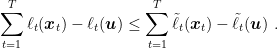
Now, define the linear (and convex) losses ${\tilde{\ell}_t({\boldsymbol x}):=\langle {\boldsymbol g}_t, {\boldsymbol x}\rangle}$ , so we have

$\displaystyle \sum_{t=1}^T \ell_t({\boldsymbol x}_t) - \ell_t({\boldsymbol u}) \leq \sum_{t=1}^T \tilde{\ell}_t({\boldsymbol x}_t) - \tilde{\ell}_t({\boldsymbol u})~.$

This is more powerful that what it seems: We upper bounded the regret with respect to the convex losses ${\ell_t}$ with a regret with respect to another sequence of linear losses. This is important because it implies that we can build online algorithms that deal only with linear losses, and through the reduction above they can be seamlessly used as OCO algorithms! Note that this not imply that this reduction is always optimal, it isn’t! But, it allows us to easily construct optimal OCO algorithms in many interesting cases.

So, we will often consider just the problem of minimizing the linear regret

$\displaystyle \text{Regret}_T({\boldsymbol u})=\sum_{t=1}^T \langle {\boldsymbol g}_t, {\boldsymbol x}_t\rangle - \sum_{t=1}^T \langle {\boldsymbol g}_t, {\boldsymbol u}\rangle, \forall {\boldsymbol u} \in V\subseteq{\mathbb R}^d~.$

This problem is called Online Linear Optimization (OLO).

Example 4 Consider the guessing game of the first class, we can solve easily it with Online Gradient Descent. Indeed, we just need to calculate the gradients, prove that they are bounded, and find a way to calculate the projection of a real number in ${[0,1]}$ So, ${\ell'_t(x)=2(x-y_t)}$ , that is bounded for ${x,y_t \in [0,1]}$ . The projection on ${[0,1]}$ is just ${\Pi_{[0,1]}(x)=\min(\max(x,0),1)}$ . With the optimal learning rate, the resulting regret would be ${O(\sqrt{T})}$ . This is worse than the one we found in the first class, showing that the reduction not always gives the best possible regret.

Example 5 Consider again the guessing game of the first class, but now change the loss function to the absolute loss of the difference: ${\ell_t(x)=|x-y_t|}$ . Now we will need to use Online Subgradient Descent, because the functions are non-differentiable. We can easily see that

$\displaystyle \partial \ell_t(x) =\begin{cases} \{1\}, & x>y_t\\ [-1,1], & x=y_t\\ \{-1\}, & x<y_t~. \end{cases}$

Again, running Online Subgradient Descent with the optimal learning rate on this problem will give us immediately a regret of ${O(\sqrt{T})}$ , without having to think to a particular strategy for it.

4. Online-to-Batch Conversion

It is a good moment to take a break from online learning theory and see some application of online learning to other domains. For example, we may wonder what is the connection between online learning and stochastic optimization. Given that Projected Online (Sub)Gradient Descent looks basically the same as Projected Stochastic (Sub)Gradient Descent, they must have something in common. Indeed, we can show that, for example, we can reduce stochastic optimization of convex functions to OCO. Let’s see how.

Theorem 8 Let ${F({\boldsymbol x})=\mathop{\mathbb E}[f({\boldsymbol x},{\boldsymbol \xi})]}$ where the expectation is w.r.t. ${{\boldsymbol \xi}}$ drawn from ${\rho}$ over some vector space ${X}$ and ${f:{\mathbb R}^d \times X\rightarrow (-\infty,+\infty]}$ is convex in the first argument. Draw ${T}$ samples ${{\boldsymbol \xi}_1,\dots,{\boldsymbol \xi}_T}$ i.i.d. from ${\rho}$ and construct the sequence of losses ${\ell_t({\boldsymbol x}) = \alpha_t f({\boldsymbol x},{\boldsymbol \xi}_t)}$ , where ${\alpha_t>0}$ are deterministic. Run any OCO algorithm over the losses ${\ell_t}$ , to construct the sequence of predictions ${{\boldsymbol x}_1,\dots,{\boldsymbol x}_{T+1}}$ . Then, we have

$\displaystyle \mathop{\mathbb E}\left[F\left(\frac{1}{\sum_{t=1}^T \alpha_t}\sum_{t=1}^T \alpha_t {\boldsymbol x}_t\right)\right] \leq F({\boldsymbol u}) + \frac{\mathop{\mathbb E}[\text{Regret}_T({\boldsymbol u})]}{\sum_{t=1}^T \alpha_t}, \ \forall {\boldsymbol u} \in {\mathbb R}^d,$

where the expectation is with respect to ${{\boldsymbol \xi}_1,\dots, {\boldsymbol \xi}_T}$ .

We will prove it next time, let’s see now an application for it: Let’s now see how to use the above theorem to transform Online Subgradient Descent in Stochastic Subgradient Descent to minimize the training error of a classifier.

Example 6 Consider a problem of binary classification, with inputs ${{\boldsymbol z}_i \in R^d}$ and outputs ${y_i \in \{-1,1\}}$ . The loss function is the hinge loss: ${f({\boldsymbol x}, ({\boldsymbol z},y)) = \max(1-y\langle {\boldsymbol z}, {\boldsymbol x}\rangle,0)}$ . Suppose that you want to minimize the training error over a training set of ${N}$ samples, ${\{({\boldsymbol z}_i,y_i)\}_{i=1}^N}$ . Also, assume the maximum L2 norm of the samples is ${R}$ . That is, we want to minimize

$\displaystyle \min_{{\boldsymbol x}} \ F({\boldsymbol x}):= \frac{1}{N}\sum_{i=1}^N \max(1-y_i\langle {\boldsymbol z}_i, {\boldsymbol x}\rangle,0)~.$

Run the reduction described in Theorem 8 for ${T}$ iterations using OGD. In each iteration, construct ${\ell_t({\boldsymbol x})=\max(1-y_t\langle {\boldsymbol z}_t, {\boldsymbol x}\rangle,0)}$ sampling a training point uniformly at random from ${1}$ to ${N}$ . Set ${{\boldsymbol x}_1=\boldsymbol{0}}$ and ${\eta=\frac{1}{R\sqrt{T}}}$ . We have that

$\displaystyle \mathop{\mathbb E}\left[F\left(\frac{1}{T}\sum_{t=1}^T {\boldsymbol x}_t\right)\right] - F({\boldsymbol x}^\star) \leq R\frac{\|{\boldsymbol x}^\star\|^2 + 1}{2\sqrt{T}}~.$

In words, we used an OCO algorithm to stochastically optimize a function, transforming the regret guarantee into a convergence rate guarantee.

Next time we will prove the Online-to-Batch theorem and show many more examples on how to use it.

5. History Bits

The specific shape of Theorem 8 is new, but I wouldn’t be surprised if it appeared somewhere in the literature. In particular, the uniform averaging is from (N. Cesa-Bianchi and A. Conconi and Gentile, C. , 2004), but was proposed for the absolute loss in (Blum, A. and Kalai, A. and Langford, J., 1999). The non-uniform averaging, that we will use next time, is from (Zhang, T., 2004), even if there it is not proposed explicitly as a online-to-batch conversion.

6. Exercises

Exercise 1 Calculate the subdifferential set of the ${\epsilon}$ -insensitive loss: ${f(x)=\max(|x-y|-\epsilon,0)}$ . It is a loss used in regression problems where we don’t want to penalize predictions ${x}$ within ${\pm \epsilon}$ of the correct value ${y}$ .

Exercise 2 Consider Projected Online Subgradient Descent for the example in the previous lecture about the failure of Follow-the-Leader: Can we use it on that problem? Would it guarantee sublinear regret? How the behaviour of the algorithm would differ from FTL?

Exercise 3 Implement the algorithm in 6 in any language you like: implementing an algorithm is the perfect way to see if you understood all the details of the algorithm.

5 Comments

Pingback: More Online-to-Batch Examples and Strong Convexity – Parameter-free Learning and Optimization Algorithms
Pingback: Adaptive Algorithms: L* bounds and AdaGrad – Parameter-free Learning and Optimization Algorithms
Pingback: Online Mirror Descent II: Regret and Mirror Version – Parameter-free Learning and Optimization Algorithms
Pingback: Online Mirror Descent III: Examples and Learning with Expert Advice – Parameter-free Learning and Optimization Algorithms
Nicolò says:

October 4, 2019 at 4:43 PM

Hi, in definition 6 for the Lipshitz functions I think there is a missing $L$ in the equation: {|f({\boldsymbol x})-f({\boldsymbol y})|\leq \|{\boldsymbol x}-{\boldsymbol y}\|

Also, in Example 6 it’s written “training set of N samples {\{({\boldsymbol x}_i,y_i)\}_{i=1}^N}”, but we said before that our inputs are {\boldsymbol z}_i \in R^d

I think I’m missing something in the second implication of Theorem 7, i.e. assuming {\|{\boldsymbol g}\|_2\leq L} then the function is $L$-Lipshitz. If we use the definition of subgradient we get

\displaystyle f({\boldsymbol x})-f({\boldsymbol y}) \leq \langle {\boldsymbol g}, \|{\boldsymbol x}-{\boldsymbol y}

why does it hold for the absolute value as well?

Thanks,

Nicolò

LikeLike

1. bremen79 says:
  
  October 4, 2019 at 6:32 PM
  
  Thanks for finding the typos! I fixed them now.
  For the proof of Theorem 7, I was indeed a bit sloppy. I changed the proof: you just do the same reasoning twice, swapping the role of x and y. Does it work now?
  
  LikeLike
  
  1. Nicolò says:
    
    October 5, 2019 at 4:47 AM
    
    Right, thank you!
    
    LikeLiked by 1 person
Pingback: Follow-The-Regularized-Leader I: Regret Equality – Parameter-free Learning and Optimization Algorithms
Pingback: Parameter-free Online Learning II: Reductions – Parameter-free Learning and Optimization Algorithms
Pingback: From Online Learning to Statistical Learning – Parameter-free Learning and Optimization Algorithms
Rotem says:

February 27, 2020 at 7:01 AM

In example 6, shouldn’t the sqrt(T) be in the numerator and not the denominator?
Thanks!

LikeLike

1. bremen79 says:
  
  February 27, 2020 at 10:32 AM
  
  I think it is correct: the regret is sqrt{T} and the online-to-batch conversion divides the regret by T, right?
  
  LikeLike

Share this:

Like this:

Related

Leave a Reply Cancel reply