From Online Learning to Statistical Learning

This post is part of the lecture notes of my class “Introduction to Online Learning” I taught at Boston University during Fall 2019.

You can find the other lectures here.

In this lecture, we will explore the link between Online Learning and and Statistical Learning Theory.

1. Agnostic PAC Learning

We now consider a different setting from what we have seen till now. We will assume that we have a prediction strategy ${\phi_{{\boldsymbol x}}}$ parametrized by a vector ${{\boldsymbol x}}$ and we want to learn the relationship between an input ${{\boldsymbol z}}$ and its associated label ${y}$ . Moreover, we will assume that ${({\boldsymbol z},y)}$ is drawn from a joint probability distribution ${\rho}$ . Also, we are equipped with a loss function that measures how good is our prediction ${\hat{y}=\phi_{{\boldsymbol x}}({\boldsymbol z})}$ compared to the true label ${y}$ , that is ${\ell(\hat{y},y)}$ . So, learning the relationship can be cast as minimizing the expected loss of our predictor

$\displaystyle \min_{{\boldsymbol x} \in V} \ \mathop{\mathbb E}_{({\boldsymbol z},y)\sim\rho}[\ell(\phi_{{\boldsymbol x}}({\boldsymbol z}), y)]~.$

In machine learning terms, the object above is nothing else than the test error and our predictor.

Note that the above setting assumes labeled samples, but we can generalize it even more considering the Vapnik’s general setting of learning, where we collapse the prediction function and the loss in a unique function. This allows, for example, to treat supervised and unsupervised learning in the same unified way. So, we want to minimize the risk

$\displaystyle \min_{{\boldsymbol x} \in V} \ \left(\text{Risk}({\boldsymbol x}):=\mathop{\mathbb E}_{{\boldsymbol \xi}\sim\rho} [f({\boldsymbol x},{\boldsymbol \xi})]\right),$

where ${\rho}$ is an unknown distribution over ${D}$ and ${f:{\mathbb R}^d \times D \rightarrow {\mathbb R}}$ is measurable w.r.t. the second argument. Also, the set ${\mathbb{F}}$ of all predictors that can be expressed by vectors ${{\boldsymbol x}}$ in ${V}$ is called the hypothesis class.

Example 1. In a linear regression task where the loss is the square loss, we have ${{\boldsymbol \xi}=({\boldsymbol z}, y) \in {\mathbb R}^d \times {\mathbb R}}$ and ${\phi_{{\boldsymbol x}}({\boldsymbol z})=\langle {\boldsymbol z},{\boldsymbol x}\rangle}$ . Hence, ${f({\boldsymbol x},{\boldsymbol \xi})=(\langle {\boldsymbol z},{\boldsymbol x}\rangle-y)^2}$ .

Example 2. In linear binary classification where the loss is the hinge loss, we have ${{\boldsymbol \xi}=({\boldsymbol z}, y) \in {\mathbb R}^d \times \{-1, 1\}}$ and ${\phi_{{\boldsymbol x}}({\boldsymbol z})=\langle {\boldsymbol z}, {\boldsymbol x}\rangle}$ . Hence, ${f({\boldsymbol x},{\boldsymbol \xi})=\max(1-y\langle {\boldsymbol z},{\boldsymbol x}\rangle,0)}$ .

Example 3. In binary classification with a neural network with the logistic loss, we have ${{\boldsymbol \xi}=({\boldsymbol x},y) \in {\mathbb R}^d \times \{-1,1\}}$ and ${\phi_{{\boldsymbol x}}}$ is the network corresponding to the weights ${{\boldsymbol x}}$ . Hence, ${f({\boldsymbol x},{\boldsymbol \xi})=\ln(1+ \exp(-y \phi_{{\boldsymbol x}}({\boldsymbol z})))}$ .

The key difficulty of the above problem is that we don’t know the distribution ${\rho}$ . Hence, there is no hope to exactly solve this problem. Instead, we are interested in understanding what is the best we can do if we have access to ${T}$ samples drawn i.i.d. from ${\rho}$ . More in details, we want to upper bound the excess risk

$\displaystyle \text{Risk}({\boldsymbol x}_T) - \min_{{\boldsymbol x}} \text{Risk}({\boldsymbol x}),$

where ${{\boldsymbol x}_T}$ is a predictor that was learned using ${T}$ samples.

It should be clear that this is just an optimization problem and we are interested in upper bounding the suboptimality gap. In this view, the objective of machine learning can be considered as a particular optimization problem.

Remark 1. Note that this is not the only way to approach the problem of learning. Indeed, the regret minimization model is an alternative model to learning. Moreover, another approach would be to try to estimate the distribution ${\rho}$ and then solve the risk minimization problem, the approach usually taken in Statistics. No approach is superior to the other and each of them has its pros and cons.

Given that we have access to the distribution ${\rho}$ through samples drawn from it, any procedure we might think to use to minimize the risk will be stochastic in nature. This means that we cannot assure a deterministic guarantee. Instead, we can try to prove that with high probability our minimization procedure will return a solution that is close to the minimizer of the risk. It is also intuitive that the precision and probability we can guarantee must depend on how many samples we draw from ${\rho}$ .

Quantifying the dependency of precision and probability of failure on the number of samples used is the objective of the Agnostic Probably Approximately Correct (PAC) framework, where the keyword “agnostic” refers to the fact that we don’t assume anything on the best possible predictor. More in details, given a precision parameter ${\epsilon}$ and a probability of failure ${\delta}$ , we are interested in characterizing the sample complexity of the hypothesis class ${\mathbb{F}}$ that is defined as the number of samples ${T}$ necessary to guarantee with probability at least ${1-\delta}$ that the best learning algorithm using the hypothesis class ${\mathbb{F}}$ outputs a solution ${{\boldsymbol x}_T}$ that has an excess risk upper bounded by ${\epsilon}$ . Note that the sample complexity does not depend on ${\rho}$ , so it is a worst-case measure w.r.t. all the possible distributions. This makes sense if you think that we know nothing about the distribution ${\rho}$ , so if your guarantee holds for the worst distribution it will also hold for any other distribution. Mathematically, we will say that the hypothesis class is agnostic PAC-learnable is such sample complexity function exists.

Definition 1. We will say that a function class ${F=\{ f({\boldsymbol x},\cdot): {\boldsymbol x}\in {\mathbb R}^d\}}$ is Agnostic-PAC-learnable if there exists an algorithm ${\mathcal{A}}$ and a function ${T(\epsilon, \delta)}$ such that when ${\mathcal{A}}$ is used with ${T\geq T(\epsilon, \delta)}$ samples drawn from ${\rho}$ , with probability at least ${1-\delta}$ the solution ${{\boldsymbol x}_T}$ returned by the algorithm has excess risk at most ${\epsilon}$ .

Note that the Agnostic PAC learning setting does not say what is the procedure we should follow to find such sample complexity. The approach most commonly used in machine learning to solve the learning problem is the so-called Empirical Risk Minimization (ERM) problem. It consist of drawing ${T}$ samples i.i.d. from ${\rho}$ and minimizing the empirical risk:

$\displaystyle \widehat{\text{Risk}}({\boldsymbol x}):=\min_{{\boldsymbol x} \in V} \frac{1}{T} \sum_{t=1}^T f({\boldsymbol x};{\boldsymbol \xi}_t)~.$

In words, ERM is nothing else than minimize the error on a training set. However, in many interesting cases we can have that ${\mathop{\mathrm{argmin}}_{{\boldsymbol x} \in V} \frac{1}{T} \sum_{t=1}^T f({\boldsymbol x};{\boldsymbol \xi}_t)}$ can be very far from the true optimum ${\mathop{\mathrm{argmin}}_{{\boldsymbol x} \in V} \mathop{\mathbb E}[f({\boldsymbol x};{\boldsymbol \xi})]}$ , even with an infinite number of samples! So, we need to modify the ERM formulation in some way, e.g., using a regularization term or a Bayesian prior of ${{\boldsymbol x}}$ , or find conditions under which ERM works.

The ERM approach is so widespread that machine learning itself is often wrongly identified with some kind of minimization of the training error. We now show that ERM is not the entire world of ML, showing that the existence of a no-regret algorithm, that is an online learning algorithm with sublinear regret, guarantee Agnostic-PAC learnability. More in details, we will show that an online algorithm with sublinear regret can be used to solve machine learning problems. This is not just a curiosity, for example this gives rise to computationally efficient parameter-free algorithms, that can be achieved through ERM only running a two-step procedure, i.e. running ERM with different parameters and selecting the best solution among them.

We already mentioned this possibility when we talked about the online-to-batch conversion, but this time we will strengthen it proving high probability guarantees rather than expectation ones.

So, we need some more bits on concentration inequalities.

2. Bits on Concentration Inequalities

We will use a concentration inequality to prove the high probability guarantee, but we will need to go beyond the sum of i.i.d.random variables. In particular, we will use the concept of martingales.

Definition 2. A sequence of random variables ${X_1, X_2, \dots}$ is called a martingale if for all ${t\geq1}$ it satisfies:

$\displaystyle \begin{aligned} &\mathop{\mathbb E}[|X_t|]< \infty, &\mathop{\mathbb E}[X_{t+1}|X_1, \dots, X_t] = X_t~. \end{aligned}$

Example 4. Consider a fair coin ${c_t}$ and a betting algorithm that bets ${|x_t|}$ money on each round on the side of the coin equal to ${\rm sign(x_t)}$ . We win or lose money 1:1, so the total money we won up to round ${t}$ is ${Z_t=\sum_{i=1}^t c_t x_t}$ . ${Z_1, \dots, Z_t}$ is a martingale. Indeed, we have

$\displaystyle \mathop{\mathbb E}[Z_t|Z_1, \dots, Z_{t-1}] =\mathop{\mathbb E}[Z_{t-1} + x_t c_t|Z_1, \dots, Z_{t-1}] =Z_{t-1} + \mathop{\mathbb E}[x_t c_t|Z_1, \dots, Z_{t-1}] =0~.$

For bounded martingales we can prove high probability guarantees as for bounded i.i.d. random variables. The following Theorem will be the key result we will need.

Theorem 3 (Hoeffding-Azuma inequality). Let ${Z_1, \dots, Z_T}$ be a martingale of ${T}$ random variables that satisfy ${|Z_t - Z_{t+1}| \leq B, t=1, \dots, T-1}$ almost surely. Then, we have

$\displaystyle \mathop{\mathbb P}[Z_T - Z_0 \geq \epsilon] \leq \exp\left(-\frac{\epsilon^2}{2 B^2 T}\right)~.$

Also, the same upper bounds hold on ${\mathop{\mathbb P}[Z_0 - Z_T \geq \epsilon]}$ .

3. From Regret to Agnostic PAC

We now show how the online-to-batch conversion we introduced before gives us high probability guarantee for our machine learning problem.

Theorem 4. Let ${\text{Risk}({\boldsymbol x})=\mathop{\mathbb E}[f({\boldsymbol x},{\boldsymbol \xi})]}$ , where the expectation is w.r.t. ${{\boldsymbol \xi}}$ drawn from ${\rho}$ with support over some vector space ${D}$ and ${f:{\mathbb R}^d \times D\rightarrow [0,1]}$ . Draw ${T}$ samples ${{\boldsymbol \xi}_1,\dots,{\boldsymbol \xi}_T}$ i.i.d. from ${\rho}$ and construct the sequence of losses ${\ell_t({\boldsymbol x}) = f({\boldsymbol x},{\boldsymbol \xi}_t)}$ . Run any online learning algorithm over the losses ${\ell_t}$ , to construct the sequence of predictions ${{\boldsymbol x}_1,\dots,{\boldsymbol x}_{T+1}}$ . Then, we have with probability at least ${1-\delta}$ , it holds that

$\displaystyle \frac{1}{T}\sum_{t=1}^T \text{Risk}({\boldsymbol x}_i) \leq \inf_{{\boldsymbol u} \in {\mathbb R}^d} \ \text{Risk}({\boldsymbol u}) + \frac{\text{Regret}_T({\boldsymbol u})}{T} + 2\sqrt{\frac{2\ln\frac{2}{\delta}}{T}}~.$

Proof: Define ${Z_t=\sum_{i=1}^t \left(\text{Risk}({\boldsymbol x}_i)-\ell_i({\boldsymbol x}_i)\right)}$ . We claim that ${Z_t}$ is a martingale. In fact, we have

$\displaystyle \mathop{\mathbb E}[\ell_t({\boldsymbol x}_t)|{\boldsymbol \xi}_1, \dots, {\boldsymbol \xi}_{t-1}] = \mathop{\mathbb E}[ f({\boldsymbol x}_t, {\boldsymbol \xi}_t)|{\boldsymbol \xi}_1, \dots, {\boldsymbol \xi}_{t-1}] = \text{Risk}({\boldsymbol x}_t),$

where we used the fact that ${{\boldsymbol x}_{t}}$ depends only on ${{\boldsymbol \xi}_1,\dots,{\boldsymbol \xi}_{t-1}}$ Hence, we have

$\displaystyle \mathop{\mathbb E}[Z_{t+1}|Z_1, \dots, Z_{t}]= Z_{t}+ \mathop{\mathbb E}[\text{Risk}({\boldsymbol x}_{t+1})-\ell_{t+1}({\boldsymbol x}_{t+1})|Z_1, \dots, Z_{t}] = Z_{t},$

that proves our claim.

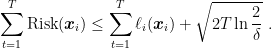
Hence, using Theorem 3, we have

$\displaystyle \mathop{\mathbb P}\left[ \sum_{t=1}^T \left(\text{Risk}({\boldsymbol x}_i)-\ell_i({\boldsymbol x}_i)\right)\geq \epsilon\right] =\mathop{\mathbb P}\left[ Z_T-Z_0\geq \epsilon\right] \leq \exp\left(-\frac{\epsilon^2}{2T}\right)~.$

This implies that, with probability at least ${1-\delta/2}$ , we have

$\displaystyle \sum_{t=1}^T \text{Risk}({\boldsymbol x}_i) \leq \sum_{t=1}^T \ell_i({\boldsymbol x}_i) + \sqrt{2T \ln \frac{2}{\delta}}~.$

or equivalently

$\displaystyle \frac{1}{T}\sum_{t=1}^T \text{Risk}({\boldsymbol x}_i) \leq \frac{1}{T}\sum_{t=1}^T \ell_i({\boldsymbol x}_i) + \sqrt{\frac{2\ln \frac{2}{\delta}}{T}}~.$

We now use the definition of regret w.r.t. any ${{\boldsymbol u}}$ , to have

$\displaystyle \frac{1}{T}\sum_{t=1}^T \ell_i({\boldsymbol x}_i) = \frac{\text{Regret}_T({\boldsymbol u})}{T} + \frac{1}{T}\sum_{t=1}^T \ell_t({\boldsymbol u})~.$

The last step is to upper bound with high probability ${\frac{1}{T}\sum_{t=1}^T \ell_t({\boldsymbol u})}$ with ${\text{Risk}({\boldsymbol u})}$ . This is easier than the previous upper bound because ${{\boldsymbol u}}$ is a fixed vector, so ${\ell_t({\boldsymbol u})}$ are i.i.d. random variables, so for sure ${Z_t=\sum_{i=1}^t \left(\text{Risk}({\boldsymbol u})-\ell_i({\boldsymbol u})\right)}$ forms a martingale. So, reasoning as above, we have that with probability at least ${1-\delta/2}$ it holds that

$\displaystyle \frac{1}{T}\sum_{t=1}^T \ell_i(u) \leq \text{Risk}({\boldsymbol u}) + \sqrt{\frac{2\ln \frac{2}{\delta}}{T}}~.$

Putting all together and using the union bound, we have the stated bound. $\Box$

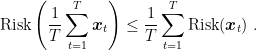
The theorem above upper bounds the average risk of the ${T}$ predictors, while we are interested in producing a single predictor. If the risk is a convex function and ${V}$ is convex, than we can lower bound the l.h.s. of the inequalities in the theorem with the risk evaluated on the average of the ${{\boldsymbol x}_t}$ . That is

$\displaystyle \text{Risk}\left(\frac{1}{T}\sum_{t=1}^T {\boldsymbol x}_t\right) \leq \frac{1}{T} \sum_{t=1}^T \text{Risk}({\boldsymbol x}_t)~.$

If the risk is not a convex function, we need a way to generate a single solution with small risk. One possibility is to construct a stochastic classifier that samples one of the ${{\boldsymbol x}_t}$ with uniform probability and predicts with it. For this classifier, we immediately have

$\displaystyle \text{Risk}(\{{\boldsymbol x}_1, \dots, {\boldsymbol x}_T\}) = \frac{1}{T} \sum_{t=1}^T \text{Risk}({\boldsymbol x}_t),$

where the expectation in the definition of the risk of the stochastic classifier is also with respect to the random index. Yet another way, is to select among the ${T}$ predictors, the one with the smallest risk. This works because the average is lower bounded by the minimum. This is easily achieved using ${T/2}$ samples for the online learning procedure and ${T/2}$ samples to generate a validation set to evaluate the solution and pick the best one. The following Theorem shows that selecting the predictor with the smallest empirical risk on a validation set will give us a predictor close to the best one with high probability.

Theorem 5. We have a finite set of predictors ${S=\{{\boldsymbol x}_1, \dots, {\boldsymbol x}_{|S|}\}}$ and a dataset of ${T}$ samples drawn i.i.d. from ${\rho}$ . Denote by ${\hat{{\boldsymbol x}}=\mathop{\mathrm{argmin}}_{{\boldsymbol x} in S} \ \widehat{\text{Risk}}({\boldsymbol x})}$ . Then, with probability at least ${1-\delta}$ , we have

$\displaystyle \text{Risk}(\hat{{\boldsymbol x}})\leq \min_{{\boldsymbol x} \in S} \ \text{Risk}({\boldsymbol x}) + \sqrt{\frac{2\ln(|S|/\delta)}{T}}~.$

Proof: We want to calculate the probability that the hypothesis that minimizes the validation error is far from the best hypothesis in the set. We cannot do it directly because we don’t have the required independence to use a concentration. Instead, we will upper bound the probability that there exists at least one function whose empirical risk is far from the risk. So, we have

$\displaystyle \mathop{\mathbb P}\left[\exists {\boldsymbol x} \in S: |\text{Risk}({\boldsymbol x})-\widehat{\text{Risk}}({\boldsymbol x})| > \frac{\epsilon}{2}\right] \leq \sum_{i=1}^{|S|} \mathop{\mathbb P}\left[|\text{Risk}({\boldsymbol x}_i)-\widehat{\text{Risk}}({\boldsymbol x}_i)| > \frac{\epsilon}{2}\right] \leq |S| \exp\left(-\frac{\epsilon^2T}{2}\right)~.$

Hence, with probability at least ${1-\delta}$ , we have that for all ${{\boldsymbol x} \in S}$

$\displaystyle |\text{Risk}({\boldsymbol x})-\widehat{\text{Risk}}({\boldsymbol x})| \leq \sqrt{\frac{2\ln(|S|/\delta)}{T}}~.$

We are now able to upper bound the risk of ${\hat{{\boldsymbol x}}}$ , just using the fact that the above applies to ${\hat{{\boldsymbol x}}}$ too. So, we have

$\displaystyle \text{Risk}(\hat{{\boldsymbol x}}) \leq \widehat{\text{Risk}}(\hat{{\boldsymbol x}}) + \epsilon/2 \leq \widehat{\text{Risk}}({\boldsymbol x}^*) + \epsilon/2 \leq \text{Risk}({\boldsymbol x}^*) +\epsilon,$

where in the last inequality we used the fact that ${\hat{{\boldsymbol x}}}$ minimizes the empirical risk. $\Box$

Using this theorem, we can use ${T/2}$ samples for the training and ${T/2}$ samples for the validation. Denoting by ${\hat{x}_T}$ the predictor with the best empirical risk on the validation set among the ${T/2}$ generated during the online procedure, we have with probability at least ${1-2 \delta}$ that

$\displaystyle \text{Risk}(\hat{{\boldsymbol x}}_T) \leq \inf_{{\boldsymbol u} \in {\mathbb R}^d} \ \text{Risk}({\boldsymbol u}) + \frac{\text{Regret}_T({\boldsymbol u})}{T} + 3\sqrt{\frac{2\ln(T/\delta)}{T}}~.$

It is important to note that with any of the above three methods to select one ${{\boldsymbol x}_t}$ among the ${T}$ generated by the online learning procedure, the sample complexity guarantee we get matches the one we would have obtained by ERM, up to polylogarithmic factors. In other words, there is nothing special about ERM compared to the online learning approach to statistical learning.

Another important point is that the above guarantee does not imply the existence of online learning algorithms with sublinear regret for any learning problem. It just says that, if it exists, it can be used in the statistical setting too.

4. History Bits

Theorem 4 is from (N. Cesa-Bianchi and A. Conconi and Gentile, C. , 2004). Theorem 5 is nothing else than the Agnostic PAC learning guarantee for ERM for hypothesis classes with finite cardinality. (N. Cesa-Bianchi and A. Conconi and Gentile, C. , 2004) gives also an alternative procedure to select a single hypothesis among the ${T}$ generated during the online procedure that does not require splitting the data in training and validation. However, the obtained guarantee matches the one we have proved.

Pingback: Almost Sure Convergence of SGD on Smooth Non-Convex Functions – Parameter-free Learning and Optimization Algorithms

Share this:

Like this:

Related

Leave a Reply Cancel reply