This post is part of the lecture notes of my class “Introduction to Online Learning” at Boston University, Fall 2019.
You can find all the lectures I published here.
1. Online-to-Batch Conversion
Last time we saw the following theorem, let’s now prove it.
Theorem 1 Let
where the expectation is w.r.t.
drawn from
over some vector space
and
is convex in the first argument. Draw
samples
i.i.d. from
, where
are deterministic. Run any OCO algorithm over the losses
, to construct the sequence of predictions
. Then, we have
where the expectation is with respect to
.
![\displaystyle \mathop{\mathbb E}\left[F\left(\frac{1}{\sum_{t=1}^T \alpha_t}\sum_{t=1}^T \alpha_t {\boldsymbol x}_t\right)\right] \leq F({\boldsymbol u}) + \frac{\mathop{\mathbb E}[\text{Regret}_T({\boldsymbol u})]}{\sum_{t=1}^T \alpha_t}, \ \forall {\boldsymbol u} \in {\mathbb R}^d,](https://s0.wp.com/latex.php?latex=%5Cdisplaystyle+%5Cmathop%7B%5Cmathbb+E%7D%5Cleft%5BF%5Cleft%28%5Cfrac%7B1%7D%7B%5Csum_%7Bt%3D1%7D%5ET+%5Calpha_t%7D%5Csum_%7Bt%3D1%7D%5ET+%5Calpha_t+%7B%5Cboldsymbol+x%7D_t%5Cright%29%5Cright%5D+%5Cleq+F%28%7B%5Cboldsymbol+u%7D%29+%2B+%5Cfrac%7B%5Cmathop%7B%5Cmathbb+E%7D%5B%5Ctext%7BRegret%7D_T%28%7B%5Cboldsymbol+u%7D%29%5D%7D%7B%5Csum_%7Bt%3D1%7D%5ET+%5Calpha_t%7D%2C+%5C+%5Cforall+%7B%5Cboldsymbol+u%7D+%5Cin+%7B%5Cmathbb+R%7D%5Ed%2C+&bg=ffffff&fg=000000&s=0&c=20201002)
![\displaystyle \label{eq:o2b_1} \mathop{\mathbb E}\left[\sum_{t=1}^T \alpha_t F({\boldsymbol x}_t)\right] = \mathop{\mathbb E}\left[ \sum_{t=1}^T \ell_t({\boldsymbol x}_t)\right]~. \ \ \ \ \ (1)](https://s0.wp.com/latex.php?latex=%5Cdisplaystyle+%5Clabel%7Beq%3Ao2b_1%7D+%5Cmathop%7B%5Cmathbb+E%7D%5Cleft%5B%5Csum_%7Bt%3D1%7D%5ET+%5Calpha_t+F%28%7B%5Cboldsymbol+x%7D_t%29%5Cright%5D+%3D+%5Cmathop%7B%5Cmathbb+E%7D%5Cleft%5B+%5Csum_%7Bt%3D1%7D%5ET+%5Cell_t%28%7B%5Cboldsymbol+x%7D_t%29%5Cright%5D%7E.+%5C+%5C+%5C+%5C+%5C+%281%29&bg=ffffff&fg=000000&s=0&c=20201002)
In fact, from the linearity of the expectation we have
![\displaystyle \mathop{\mathbb E}\left[ \sum_{t=1}^T \ell_t({\boldsymbol x}_t)\right] = \sum_{t=1}^T \mathop{\mathbb E}\left[\ell_t({\boldsymbol x}_t)\right]~.](https://s0.wp.com/latex.php?latex=%5Cdisplaystyle+%5Cmathop%7B%5Cmathbb+E%7D%5Cleft%5B+%5Csum_%7Bt%3D1%7D%5ET+%5Cell_t%28%7B%5Cboldsymbol+x%7D_t%29%5Cright%5D+%3D+%5Csum_%7Bt%3D1%7D%5ET+%5Cmathop%7B%5Cmathbb+E%7D%5Cleft%5B%5Cell_t%28%7B%5Cboldsymbol+x%7D_t%29%5Cright%5D%7E.+&bg=ffffff&fg=000000&s=0&c=20201002)
Then, from the law of total expectation, we have
![\displaystyle \mathop{\mathbb E}\left[\ell_t({\boldsymbol x}_t)\right] = \mathop{\mathbb E}\left[\mathop{\mathbb E}[\ell_t({\boldsymbol x}_t)|{\boldsymbol \xi}_1, \dots, {\boldsymbol \xi}_{t-1}\right] = \mathop{\mathbb E}\left[\mathop{\mathbb E}[\alpha_t f({\boldsymbol x}_t, {\boldsymbol \xi}_t)|{\boldsymbol \xi}_1, \dots, {\boldsymbol \xi}_{t-1}]\right] = \mathop{\mathbb E}\left[\alpha_t F({\boldsymbol x}_t)\right],](https://s0.wp.com/latex.php?latex=%5Cdisplaystyle+%5Cmathop%7B%5Cmathbb+E%7D%5Cleft%5B%5Cell_t%28%7B%5Cboldsymbol+x%7D_t%29%5Cright%5D+%3D+%5Cmathop%7B%5Cmathbb+E%7D%5Cleft%5B%5Cmathop%7B%5Cmathbb+E%7D%5B%5Cell_t%28%7B%5Cboldsymbol+x%7D_t%29%7C%7B%5Cboldsymbol+%5Cxi%7D_1%2C+%5Cdots%2C+%7B%5Cboldsymbol+%5Cxi%7D_%7Bt-1%7D%5Cright%5D+%3D+%5Cmathop%7B%5Cmathbb+E%7D%5Cleft%5B%5Cmathop%7B%5Cmathbb+E%7D%5B%5Calpha_t+f%28%7B%5Cboldsymbol+x%7D_t%2C+%7B%5Cboldsymbol+%5Cxi%7D_t%29%7C%7B%5Cboldsymbol+%5Cxi%7D_1%2C+%5Cdots%2C+%7B%5Cboldsymbol+%5Cxi%7D_%7Bt-1%7D%5D%5Cright%5D+%3D+%5Cmathop%7B%5Cmathbb+E%7D%5Cleft%5B%5Calpha_t+F%28%7B%5Cboldsymbol+x%7D_t%29%5Cright%5D%2C+&bg=ffffff&fg=000000&s=0&c=20201002)
where we used the fact that 

It remains only to use Jensen’s inequality, using the fact that 
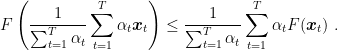
Dividing the regret by 

In example last time, we had to use a constant learning rate to be able to minimize the training error over the entire space 
Example 1 Consider the same setting of the previous example, and let’s change the way in which the construct the online losses. Now use
and step size
. Hence, we have
where we used
.
![\displaystyle \mathop{\mathbb E}\left[F\left(\sum_{t=1}^T \frac{1}{R\sqrt{t}} {\boldsymbol x}_t\right)\right] - F({\boldsymbol x}^\star) \leq \frac{\|{\boldsymbol x}^\star\|_2^2}{2\sum_{t=1}^T \frac{1}{R\sqrt{t}}} +\frac{1}{2 \sum_{t=1}^T \frac{1}{R\sqrt{t}}} \sum_{t=1}^T \frac{1}{t} \leq R\frac{\|{\boldsymbol x}^\star\|_2^2+1+\ln T}{4 \sqrt{T+1}-4},](https://s0.wp.com/latex.php?latex=%5Cdisplaystyle+%5Cmathop%7B%5Cmathbb+E%7D%5Cleft%5BF%5Cleft%28%5Csum_%7Bt%3D1%7D%5ET+%5Cfrac%7B1%7D%7BR%5Csqrt%7Bt%7D%7D+%7B%5Cboldsymbol+x%7D_t%5Cright%29%5Cright%5D+-+F%28%7B%5Cboldsymbol+x%7D%5E%5Cstar%29+%5Cleq+%5Cfrac%7B%5C%7C%7B%5Cboldsymbol+x%7D%5E%5Cstar%5C%7C_2%5E2%7D%7B2%5Csum_%7Bt%3D1%7D%5ET+%5Cfrac%7B1%7D%7BR%5Csqrt%7Bt%7D%7D%7D+%2B%5Cfrac%7B1%7D%7B2+%5Csum_%7Bt%3D1%7D%5ET+%5Cfrac%7B1%7D%7BR%5Csqrt%7Bt%7D%7D%7D+%5Csum_%7Bt%3D1%7D%5ET+%5Cfrac%7B1%7D%7Bt%7D+%5Cleq+R%5Cfrac%7B%5C%7C%7B%5Cboldsymbol+x%7D%5E%5Cstar%5C%7C_2%5E2%2B1%2B%5Cln+T%7D%7B4+%5Csqrt%7BT%2B1%7D-4%7D%2C+&bg=ffffff&fg=000000&s=0&c=20201002)
I stressed the fact that the only meaningful way to define a regret is with respect to an arbitrary point in the feasible set. This is obvious in the case we consider unconstrained OLO, because the optimal competitor is unbounded. But, it is also true in unconstrained OCO. Let’s see an example of this.
Example 2 Consider a problem of binary classification, with inputs
and outputs
. The loss function is the logistic loss:
. Suppose that you want to minimize the training error over a training set of
samples,
. Also, assume the maximum L2 norm of the samples is
. That is, we want to minimize
So, run the reduction described in Theorem 1 for
sampling a training point uniformly at random from
to
and
. We have that
In words, we will be
away from the optimal value of regularized empirical risk minimization problem, where the weight of the regularization is
would be vacuous. On the other hand, our guarantee above still make perfectly sense.

![\displaystyle \mathop{\mathbb E}\left[F\left(\frac{1}{T}\sum_{t=1}^T {\boldsymbol x}_t\right)\right] \leq \frac{R}{2\sqrt{T}} + \min_{{\boldsymbol u} \in R^d} F({\boldsymbol u}) + R\frac{\|{\boldsymbol u}\|^2}{2\sqrt{T}}~.](https://s0.wp.com/latex.php?latex=%5Cdisplaystyle+%5Cmathop%7B%5Cmathbb+E%7D%5Cleft%5BF%5Cleft%28%5Cfrac%7B1%7D%7BT%7D%5Csum_%7Bt%3D1%7D%5ET+%7B%5Cboldsymbol+x%7D_t%5Cright%29%5Cright%5D+%5Cleq+%5Cfrac%7BR%7D%7B2%5Csqrt%7BT%7D%7D+%2B+%5Cmin_%7B%7B%5Cboldsymbol+u%7D+%5Cin+R%5Ed%7D+F%28%7B%5Cboldsymbol+u%7D%29+%2B+R%5Cfrac%7B%5C%7C%7B%5Cboldsymbol+u%7D%5C%7C%5E2%7D%7B2%5Csqrt%7BT%7D%7D%7E.+&bg=ffffff&fg=000000&s=0&c=20201002)
Note that the above examples only deal with training error. However, there is a more interesting application of the online-to-batch conversion, that is to directly minimize the generalization error.
Example 3 Consider the same setting of Example 1, but now consider the case that we want to minimize the true risk, that is
where
. Our Theorem 1 still applies as is. Indeed, draw
. We obtain that
Note the fact that the risk will be close to the best regularized solution, even if we didn’t use any regularizer! The presence of the regularizer is due to OSD and we will be able to change it to other regularizer when we will see Online Mirror Descent.
![\displaystyle \min_{{\boldsymbol x} \in {\mathbb R}^d} \ \text{Risk}({\boldsymbol x}):=\mathop{\mathbb E}[\max(1-y\langle {\boldsymbol z}, {\boldsymbol x}\rangle,0)],](https://s0.wp.com/latex.php?latex=%5Cdisplaystyle+%5Cmin_%7B%7B%5Cboldsymbol+x%7D+%5Cin+%7B%5Cmathbb+R%7D%5Ed%7D+%5C+%5Ctext%7BRisk%7D%28%7B%5Cboldsymbol+x%7D%29%3A%3D%5Cmathop%7B%5Cmathbb+E%7D%5B%5Cmax%281-y%5Clangle+%7B%5Cboldsymbol+z%7D%2C+%7B%5Cboldsymbol+x%7D%5Crangle%2C0%29%5D%2C+&bg=ffffff&fg=000000&s=0&c=20201002)
![\displaystyle \mathop{\mathbb E}\left[\text{Risk}\left(\frac{1}{T}\sum_{t=1}^T {\boldsymbol x}_t\right)\right] \leq \min_{{\boldsymbol u} \in {\mathbb R}^d} \text{Risk}({\boldsymbol u}) + R\frac{\|{\boldsymbol u}\|^2 + 1}{2\sqrt{T}}~.](https://s0.wp.com/latex.php?latex=%5Cdisplaystyle+%5Cmathop%7B%5Cmathbb+E%7D%5Cleft%5B%5Ctext%7BRisk%7D%5Cleft%28%5Cfrac%7B1%7D%7BT%7D%5Csum_%7Bt%3D1%7D%5ET+%7B%5Cboldsymbol+x%7D_t%5Cright%29%5Cright%5D+%5Cleq+%5Cmin_%7B%7B%5Cboldsymbol+u%7D+%5Cin+%7B%5Cmathbb+R%7D%5Ed%7D+%5Ctext%7BRisk%7D%28%7B%5Cboldsymbol+u%7D%29+%2B+R%5Cfrac%7B%5C%7C%7B%5Cboldsymbol+u%7D%5C%7C%5E2+%2B+1%7D%7B2%5Csqrt%7BT%7D%7D%7E.+&bg=ffffff&fg=000000&s=0&c=20201002)
2. Can We Do Better Than 
Let’s now go back to online convex optimization theory. The example in the first class showed us that it is possible to get logarithmic regret in time. However, we saw that we get only 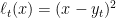
![{[0,1]}](https://s0.wp.com/latex.php?latex=%7B%5B0%2C1%5D%7D&bg=ffffff&fg=000000&s=0&c=20201002)
The key concept we will need is the one of strong convexity.
3. Convex Analysis Bits: Strong Convexity
Here, we introduce a stronger concept of convexity, that allows to build better lower bound to a function. Instead of the linear lower bound achievable through the use of subgradients, we will make use of quadratic lower bound.
Definition 2 Let
. A proper function
is
-strongly convex over a convex set
w.r.t.
if

Remark 1 You might find another definition of strong convexity, that resembles the one of convexity. However, it is easy to show that these two definitions are equivalent.
Note that the any convex function is 


In words, the definition above tells us that a strongly convex function can be lower bounded by a quadratic, where the linear term is the usual one constructed through the subgradient, and the quadratic term depends on the strong convexity. Hence, we have a tighter lower bound to the function w.r.t. simply using convexity. This is what we would expect using a Taylor expansion on a twice-differentiable convex function and lower bounding the smallest eigenvalue of the Hessian. Indeed, we have the following Theorem
Theorem 3 (S. Shalev-Shwartz, 2007, Lemma 14) Let
convex and
twice differentiable. Then, a sufficient condition for
w.r.t.
we have
, where
is the Hessian matrix of
at
.
However, here there is the important difference that we do not assume the function to be twice differentiable. Indeed, we don’t even need plain differentiability. Hence, the use of the subgradient implies that this lower bound does not have to be uniquely determined, as in the next Example.

 .
.Example 4 Consider the strongly convex function
.
We also have the following easy but useful property on the sum of strong convex functions.
Theorem 4 Let
be
-strongly convex and
a
-strongly convex function in a non-empty convex set
w.r.t.
. Then,
is
-strongly convex in
Proof: Note that the assumption on
Example 5 Let
. Using Theorem 3, we have that
4. Online Subgradient Descent for Strongly Convex Losses
Theorem 5 Assume that the functions
are
-strongly convex w.r.t
, where
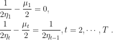
. Use OSD with stepsizes equal to
. Then, for any
, we have the following regret guarantee
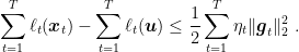
Proof: From the assumption of

From the fact that
Hence, use Lemma 2 in Lecture 3 and sum from 

Observing that the first sum on the left hand side is a telescopic sum, we have the stated bound.
Remark 2 Notice that the theorem requires a bounded domain, otherwise the loss functions will not be Lipschitz given that they are also strongly convex.
Corollary 6 Under the assumptions of Theorem 5, if in addiction we have
and
-Lipschitz w.r.t.
, then we have
Remark 3 Corollary 6 does not imply that for any finite
. Instead, asymptotically the regret in Corollary 6 is always better than to one of OSD with Lipschitz losses.
Example 6 Consider once again the example in the first class:
-strongly convex w.r.t.
. Hence, setting
and
gives a regret of
.
Let’s now use again the online-to-batch conversion on strongly convex stochastic problems.
Example 7 As done before, we can use the online-to-batch conversion to use Corollary 6 to obtain stochastic subgradient descent algorithms for strongly convex stochastic functions. For example, consider the classic Support Vector Machine objective
or any other regularized formulation like regularized logistic regression:
where
,
, and
. First, notice that the minimizer of both expressions has to be in the L2 ball of radius proportional to
(proof left as exercise). Hence, we can set
or
results in
However, we can do better! Indeed,
or
results in
-strongly convex loss functions. Using Corollary 6, we have that
and Theorem 1 gives immediately
that is asymptotically better because it does not have the logarithmic term.
![\displaystyle \mathop{\mathbb E}\left[F\left(\frac{1}{T}\sum_{t=1}^T {\boldsymbol x}_t\right)\right] - \min_{{\boldsymbol x}} \ F({\boldsymbol x}) \leq O\left(\frac{\ln T}{ \lambda T}\right)~.](https://s0.wp.com/latex.php?latex=%5Cdisplaystyle+%5Cmathop%7B%5Cmathbb+E%7D%5Cleft%5BF%5Cleft%28%5Cfrac%7B1%7D%7BT%7D%5Csum_%7Bt%3D1%7D%5ET+%7B%5Cboldsymbol+x%7D_t%5Cright%29%5Cright%5D+-+%5Cmin_%7B%7B%5Cboldsymbol+x%7D%7D+%5C+F%28%7B%5Cboldsymbol+x%7D%29+%5Cleq+O%5Cleft%28%5Cfrac%7B%5Cln+T%7D%7B+%5Clambda+T%7D%5Cright%29%7E.+&bg=ffffff&fg=000000&s=0&c=20201002)
![\displaystyle \mathop{\mathbb E}\left[F\left(\frac{2}{T(T+1)}\sum_{t=1}^T t\, {\boldsymbol x}_t\right)\right] - \min_{{\boldsymbol x}} \ F({\boldsymbol x}) \leq O\left(\frac{1}{\lambda T}\right),](https://s0.wp.com/latex.php?latex=%5Cdisplaystyle+%5Cmathop%7B%5Cmathbb+E%7D%5Cleft%5BF%5Cleft%28%5Cfrac%7B2%7D%7BT%28T%2B1%29%7D%5Csum_%7Bt%3D1%7D%5ET+t%5C%2C+%7B%5Cboldsymbol+x%7D_t%5Cright%29%5Cright%5D+-+%5Cmin_%7B%7B%5Cboldsymbol+x%7D%7D+%5C+F%28%7B%5Cboldsymbol+x%7D%29+%5Cleq+O%5Cleft%28%5Cfrac%7B1%7D%7B%5Clambda+T%7D%5Cright%29%2C+&bg=ffffff&fg=000000&s=0&c=20201002)
5. History Bits
The logarithmic regret in Corollary 6 was shown for the first time in the seminal paper (Hazan, E. and Kalai, A. and Kale, S. and Agarwal, A., 2006). The general statement in Theorem 5 was proven by (Hazan, E. and Rakhlin, A. and Bartlett, P. L., 2008).
As we said last time, the non-uniform averaging of Example 1 is from (Zhang, T., 2004), even if there it is not proposed explicitly as an online-to-batch conversion. Instead, the non-uniform averaging of Example 7 is from (Lacoste-Julien, S. and Schmidt, M. and Bach, F., 2012), but again there is not proposed as an online-to-batch conversion. The basic idea of solving the problem of SVM with OSD and online-to-batch conversion of Example 7 was the Pegasos algorithm (S. Shalev-Shwartz and Y. Singer and N. Srebro, 2007), for many years the most used optimizer for SVMs.
A more recent method to do online-to-batch conversion has been introduced in (Cutkosky, 2019). The new method allows to prove the convergence of the last iterate rather than the one of the weighted average, with a small change in the online learning algorithm.
6. Exercises
Exercise 1 Prove that OSD in Example 6 with
is exactly the Follow-the-Leader strategy for that particular problem.
Exercise 2 Prove that
is
Exercise 3 (Difficult) Prove that
is
-strongly convex w.r.t.
where
.

There is a nice recent paper by Ashok Cutkosky that deals with online-to-batch conversion in an elegant way: http://proceedings.mlr.press/v97/cutkosky19a/cutkosky19a.pdf
LikeLike
Hi David, nice to see you here 🙂
Good point, I forgot about that paper! I’ll add it to the references.
LikeLike
Hi! Found some typos: in Example 2 “training set of N samples, {x_i, y_i}” should be “{z_i, y_i}” ; in Example 3 the min should be over x \in R^d ; in Example 7 you first mention Corollary 4 and then Theorem 4 (which I guess are the same) even if neither of them are formally stated anywhere (though there is a reference pointing to a bound).
I have a doubt regarding the proof of Theorem 5. In the end we have a telescopic sum, thus we should have the first and the last term. Now, the last term should be negative so we can get rid of it, but the first term should be $ \frac{1}{2 \eta_0} \| x_1 – u \| $. I wanted to ask how is $ \eta_0 $ defined and what happens to this first term?
Thanks,
Nicolò
LikeLike
I fixed the typos, thanks a lot! (The missing corollary was actually an error in my version of latex2wp: It should have affected any other corollary I published, I’ll have to doublecheck…)
In Theorem 5, I added some more details to the proof and avoided to define 1/eta_0=0, it should be fine now.
LikeLike
Hi. Cool stuff, it’s great someone wrote in a less abstract and exotic way.
Qestion: shouldn’t the ball in example 7 be just 1 over lambda without the square root? In theorem 5 there is a typo (subscript of \mu is t instead of i).
LikeLike
Thanks for finding the typo, fixed it now.
Regarding the ball in example 7, I think it is correct. The trick is to observe that the minimum is smaller than any other value, in particular it is smaller than the objective function in the null vector. Let me know if you see how to do it.
LikeLiked by 1 person
Yes, I see it. But am I correct that comparing gradient to 0 and upper-bounding the norm by L from Lipschitz we get 1/lambda and this should tighter for bigger lambdas >1? (which probably is irrelevant considering mostly used lambda values are lower).
LikeLike
I am not sure I see how to do it: || lambda x^* + \nabla \ell_t(x^\star)|| \geq 0?
LikeLike
From first order optimality condition we get x = -\nabla \ell(x) /\lambda which implies \|x\|_* \|\nabla \ell(x)/\lambda \|_* and it’s \leq L/\lambda since both losses are Lipschitz. Ooor did I do something terribly wrong?
LikeLike
Ah yes, now I understand what you mean! It is a good point indeed, I don’t think I ever saw it. Probably the reason is that, as you say, people only care about small lambda. However, a practical implementation could definitely use this observation and take the min between the two estimated radiuses.
LikeLiked by 1 person
Dear Prof. Orabona,
I am a little confused about Theorem 1. In the statement you have mentioned that the terms $(\alpha_t)_{t \geq 1}$ are `deterministic. Later in the proof, you have mentioned that $x_t$ and $\alpha_t$ `depend only on $x_1, \ldots, \xi_{t-1}$’. But since $\xi_i$ are random variables, doesn’t that make $\alpha_t$ random as well? So, why is the term $\sum_{t=1}^T \alpha_t$ in the right-hand-side of the statement in Theorem 1 not within expectation?
Thanks!
LikeLiked by 1 person
Good catch! It is actually a typo: I didn’t want to deal with stochastic alpha_t, I have fixed now the post and I’ll fix the arxiv in the next release. Thanks!
LikeLike