Multi-scale Expert Algorithm to Tune Learning Rates

This time we consider an application of Online Mirror Descent (OMD) to the problem of prediction with multi-scale expert advice.

In this setting, at each time step {t}, an algorithm selects a probability distribution {{\boldsymbol x}_t} over a set of {d} experts (or actions). After observing a loss vector {{\boldsymbol g}_t \in {\mathbb R}^d}, the algorithm incurs a loss of {\langle {\boldsymbol g}_t, {\boldsymbol x}_t \rangle}. The goal is to minimize the regret with respect to the best single expert in hindsight. However, unlike in the usual learning with expert advice setting, here the losses associated with different experts can have vastly different scales. For example, one expert might correspond to a low-risk, low-reward strategy with losses in {[-0.1, 0.1]}, while another might be a high-risk, high-reward strategy with losses in {[-100, 100]}. Thus, we would like to prove a regret guarantee that depends on the range of the best coordinate.

A standard and effective algorithm for this problem is the Exponentiated Gradient (EG) algorithm, which we saw previously as an instance of OMD. The EG algorithm has a regret bound that scales with the largest range of the loss coordinates, so it is not suitable for this problem. We need a different algorithm.

In this setting, we assume that we have prior knowledge of the approximate scale of losses for each expert. Specifically, for each expert {i \in \{1, \dots, d\}}, we know a value {c_i > 0} such that the loss {g_{t,i}} is guaranteed to be in the range {[-c_i, c_i]} for all {t}. The goal is to leverage this scale information to achieve better regret bounds.


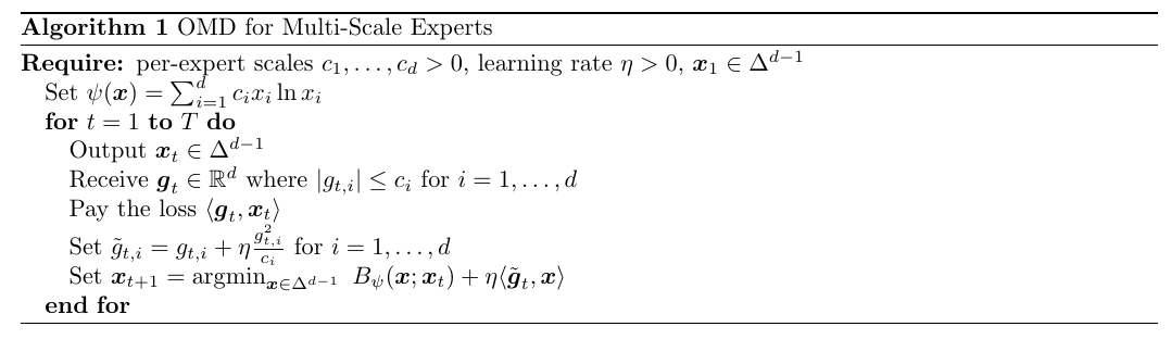
Here, we derive an algorithm for this setting as an instance of OMD with a specific choice of surrogate losses. In particular, we run OMD with distance generating function {\psi({\boldsymbol x})=\sum_{i=1}^d c_i x_i \ln x_i} on the shifted losses {\tilde{g}_{t,i}=g_{t,i}+\eta\frac{g_{t,i}^2}{c_i}}, see Algorithm 1.

Theorem 1. Let {c_1, \dots, c_d>0} such that {|g_{t,i}|\leq c_i} for all {t=1, \dots T} and {i=1, \dots d}. In Algorithm 1, set {\eta\leq \frac{1}{5}}. Then, we have

\displaystyle \sum_{t=1}^T \langle {\boldsymbol g}_t, {\boldsymbol x}_t- {\boldsymbol u}\rangle \leq \frac{B_\psi({\boldsymbol u};{\boldsymbol x}_1)}{\eta} + \eta \sum_{t=1}^T \sum_{i=1}^d \frac{u_{i} g_{t,i}^2}{c_i}, \quad \forall {\boldsymbol u} \in \Delta^{d-1}~.

Proof: First, observe that

\displaystyle |\tilde{g}_{t,i}| \leq |g_{t,i}| \left(1+ \eta \right)~. \label{eq:proof_multi-scale_eq1} \ \ \ \ \ (1)

Using the local norm regret upper bound for OMD, we obtain

\displaystyle \sum_{t=1}^T \langle \tilde{{\boldsymbol g}}_t, {\boldsymbol x}_t- {\boldsymbol u}\rangle \leq \frac{B_\psi({\boldsymbol u};{\boldsymbol x}_1)}{\eta} + \frac{\eta}{2} \sum_{t=1}^T \sum_{i=1}^d \frac{z_{t,i} \tilde{g}_{t,i}^2}{c_i}, \quad \forall {\boldsymbol u} \in \Delta^{d-1},

where {{\boldsymbol z}_{t}} is between {{\boldsymbol x}_t} and {{\boldsymbol x}'_{t+1} = \mathop{\mathrm{argmin}}_{{\boldsymbol x} \in {\mathbb R}^d_{\geq 0}} \ B_\psi({\boldsymbol x}; {\boldsymbol x}_t)+ \eta\langle \tilde{{\boldsymbol g}}_t, {\boldsymbol x}\rangle}. Using (1), we have that

\displaystyle x'_{t+1,i} = x_{t,i} \exp\left(-\eta\frac{\tilde{g}_{t,i}}{c_{i}}\right) \leq x_{t,i} \exp\left(\eta+\eta^2\right)~.

So, we can upper bound each {z_{t,i}} with {\exp\left(\eta+\eta^2\right) x_{t,i}}.

Using again (1), we have that the right hand side of the regret upper bound becomes

\displaystyle \frac{B_\psi({\boldsymbol u};{\boldsymbol x}_1)}{\eta} + \frac12 \exp\left(\eta+\eta^2\right)\left(1+\eta\right)^2 \eta \sum_{t=1}^T \sum_{i=1}^d \frac{x_{t,i} g_{t,i}^2}{c_i}~.

Observe that {\eta\leq \frac{1}{5}}, so we have

\displaystyle \frac{1}{2} \exp\left(\eta+\eta^2\right)\left(1+\eta\right)^2 \leq 1~.

So, we obtain

\displaystyle \begin{aligned} \sum_{t=1}^T \langle {\boldsymbol g}_t, {\boldsymbol x}_t- {\boldsymbol u}\rangle + \sum_{t=1}^T \sum_{i=1}^d \eta \frac{g_{t,i}^2}{c_i} (x_{t,i}-u_i) &= \sum_{t=1}^T \langle \tilde{{\boldsymbol g}}_t, {\boldsymbol x}_t- {\boldsymbol u}\rangle\\ &\leq \frac{B_\psi({\boldsymbol u};{\boldsymbol x}_1)}{\eta} + \eta \sum_{t=1}^T \sum_{i=1}^d \frac{x_{t,i} g_{t,i}^2}{c_i}, \quad \forall {\boldsymbol u} \in \Delta^{d-1}~. \end{aligned}

Simplifying, we have the stated result. \Box

Let’s now see how we can choose the prior {\pi} and the initial point {{\boldsymbol x}_1 \in \Delta^{d-1}}. First, let’s calculate the value of the Bregman divergence:

\displaystyle \begin{aligned} B_\psi({\boldsymbol u};{\boldsymbol x}_1) &=\sum_{i=1}^d c_i u_i \ln u_i-\sum_{i=1}^d c_i x_{1,i} \ln x_{1,i} - \sum_{i=1}^d c_i (\ln x_{1,i}+1)(u_i-x_{1,i})\\ &=\sum_{i=1}^d c_i u_i \ln \frac{u_i}{x_{1,i}} - \sum_{i=1}^d c_i u_i + \sum_{i=1}^d c_i x_{1,i}~. \end{aligned}

Define {c_{\min}=\min_i \ c_i}, {c_{\max}=\max_i \ c_i}, and {i_{\min}} to be any index in {\mathop{\mathrm{argmin}}_i \ c_i}. If we set {{\boldsymbol u}={\boldsymbol e}_j}, we have

\displaystyle B_\psi({\boldsymbol u};{\boldsymbol x}_1) = c_j \ln \frac{1}{x_{1,j}} + \sum_{i=1}^d c_i x_{1,i} - c_j~.

Now, set {x_{1,i} = \frac{c_{\min}}{c_i} \pi_i} for {i\neq i_{\min}} and {x_{1,i_{\min}}=1-\sum_{i\neq i_{\min}} x_{1,i}}. Also, set {\pi_i = \frac{c_i}{\sum_{j=1}^d c_j}}. In this way, for {j\neq i_{\min}}, we have

\displaystyle \begin{aligned} B_\psi({\boldsymbol u};{\boldsymbol x}_1) &= c_j \ln \frac{1}{x_{1,j}} + \sum_{i=1}^d c_i x_{1,i} - c_j\\ &= c_j \ln \frac{c_j}{ c_{\min} \pi_j} + c_{\min} (1-\pi_{i_{\min}}) + c_{\min} x_{1,i_{\min}}- c_j\\ &\leq c_j \ln \frac{c_j}{ c_{\min} \pi_j} + 2 c_{\min} - c_j\\ &\leq c_j \ln \frac{c_j}{ c_{\min} \pi_j} + c_j\\ &= c_j \ln \frac{\sum_{k=1}^d c_k}{ c_{\min} } + c_j~. \end{aligned}

On the other hand, for {j=i_{\min}}, we have

\displaystyle x_{1,i_{\min}} = 1-\sum_{i\neq i_{\min}} x_{1,i} \geq 1-\sum_{i\neq i_{\min}} \pi_{i} = \pi_{i_{\min}} = \frac{ c_{\min} }{\sum_{k=1}^d c_k}~.

Hence, the previous bound also holds for all {j}. In this case, choosing {\eta=\frac{1}{5+\frac{\sqrt{T}}{\sqrt{1+\ln \frac{\sum_{i=1}^d c_i}{c_{\min}}}}}\leq \frac{1}{5}}, we have

\displaystyle \sum_{t=1}^T \langle {\boldsymbol g}_t, {\boldsymbol x}_t- {\boldsymbol e}_j\rangle \leq 2 c_j \sqrt{T \left(1+\ln \frac{\sum_{i=1}^d c_{i}}{ c_{\min} }\right)} + 5 c_j \left(1+\ln \frac{\sum_{i=1}^d c_{i}}{ c_{\min} }\right), \quad \forall j=1, \dots, d~.

Note that if {c_1=c_2=\dots=c_d} then {\ln \frac{\sum_{i=1}^d c_{i}}{ c_{\min} }=\ln d}, so we recover the bound of the EG algorithm, up to constant factors. Instead, if the scale of the losses is different, we still pay the scale of the best expert, instead of paying the biggest scale.

1. Tuning the Learning Rate using a Multi-scale Algorithm

We now show an interesting application of the multi-scale expert algorithm.

In our analysis of Online Subgradient Descent (OSD), we have seen that the choice of the learning rate {\eta_t} is critical for performance. For instance, with a constant learning rate {\eta}, the optimal choice that minimizes the regret bound is {\eta^\star = \frac{\|{\boldsymbol u}-{\boldsymbol x}_1\|_2}{\sqrt{\sum_{t=1}^T \|{\boldsymbol g}_t\|_2^2}}}, which unfortunately depends on the competitor {{\boldsymbol u}} and the entire sequence of future gradients. One might be tempted to use a grid of learning rates and select the best one in hindsight, but unfortunately this is not a valid online learning procedure.

In this section, we demonstrate how to use a multi-scale expert algorithm to design a meta-algorithm that automatically adapts to the best learning rate from a given set, paying only a small price in the regret. The core idea is to treat each instance of an online learning algorithm with a fixed learning rate as an “expert”. We then use a multi-scale expert algorithm to combine the predictions of these experts. The resulting ensemble algorithm will have a regret guarantee that is close to the regret of the best expert—and thus the best learning rate—in hindsight.

Let us consider running {N} parallel instances of the OSD algorithm, each with a different learning rate {\eta^{(i)}} for {i=1, \dots, N}. At each round {t}, each OSD instance {i} produces a prediction {{\boldsymbol x}_t^{(i)}}. We can view these {N} predictions as advice from {N} experts. Our goal is to combine them into a single prediction {{\boldsymbol x}_t} that performs nearly as well as the best prediction {{\boldsymbol x}_t^{(i^\star)}} from the best OSD instance {i^\star}.

A straightforward approach would be to compute the loss {\ell_t({\boldsymbol x}_t^{(i)})} for each expert {i} and use this as the loss vector for the Multi-scale Expert algorithm. However, this would require computing {N} separate subgradients {{\boldsymbol g}_t^{(i)} \in \partial\ell_t({\boldsymbol x}_t^{(i)})} at each round, which can be computationally expensive.

To create an efficient algorithm that requires only one subgradient evaluation per round, we can use the following linearization technique. The controller algorithm forms its combined prediction {{\boldsymbol x}_t = \sum_{i=1}^N p_{t,i} {\boldsymbol x}_t^{(i)}}. We then receive a single subgradient {{\boldsymbol g}_t \in \partial\ell_t({\boldsymbol x}_t)} at this combined point. This single subgradient is then used to define a linear surrogate loss, {\tilde{\ell}_t({\boldsymbol x}) = \langle {\boldsymbol g}_t, {\boldsymbol x} \rangle}, which is passed to all expert algorithms and to the controller algorithm.

Because all experts receive the same linear loss function, they all use the same subgradient {{\boldsymbol g}_t} for their updates. The loss for the {i}-th expert, used by the multi-scale expert algorithm, is simply {\langle {\boldsymbol g}_t, {\boldsymbol x}_t^{(i)} \rangle}. This procedure is summarized in Algorithm 2.


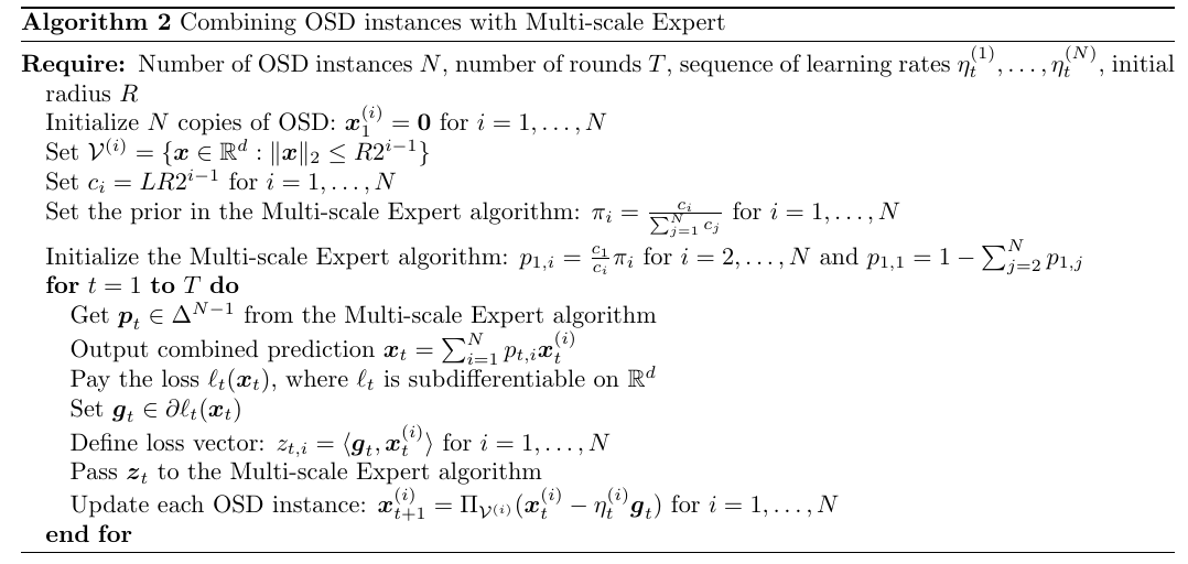
We can now prove a regret bound for this ensemble algorithm.

Theorem 2. Let {R>0} and fix {T} the number of rounds. With the notation in Algorithm 2, assume that the losses {\ell_t} are {L}-Lipschitz with respect to {\|\cdot\|_2}. Let {\eta^{(i)}_t=\frac{R 2^{i-1}}{L \sqrt{T}}} be the set of learning rates for the OSD experts, {N = \lceil \log_2\sqrt{T}\rceil+1}, and the learning rate of the Multi-scale Expert algorithm {\alpha=\frac{\sqrt{1+\ln(2^N-1)}}{5\sqrt{1+\ln(2^N-1)}+\sqrt{T}}}. Then, Algorithm 2 satisfies

\displaystyle \sum_{t=1}^T (\ell_t({\boldsymbol x}_t) - \ell_t({\boldsymbol u})) \leq \max(2\|{\boldsymbol u}\|_2, R) L \left[\sqrt{T}\left(1 + 2\sqrt{3+\ln\sqrt{T}}\right)+ 15+5\ln \sqrt{T}\right], \quad \forall {\boldsymbol u}: \|{\boldsymbol u}\|_2 \leq R \sqrt{T} ~.

Proof: The choice of {N} ensures that for any {{\boldsymbol u}} such that {\|{\boldsymbol u}\|_2\leq R \sqrt{T}} there exists an expert {j_{{\boldsymbol u}}\in\{1,\dots,N\}} such that {\|{\boldsymbol u}\|_2 \leq R2^{j_{{\boldsymbol u}}-1} \leq \max(2\|{\boldsymbol u}\|_2,R)}. Indeed, if {\|{\boldsymbol u}\|_2\leq R} we take {j_{{\boldsymbol u}}=1}, while otherwise we take {j_{{\boldsymbol u}}=\left\lceil\log_2 \frac{\|{\boldsymbol u}\|_2}{R}\right\rceil+1}.

By the definition of subgradient, the regret of the ensemble algorithm can be bounded by the regret on the linearized losses:

\displaystyle \sum_{t=1}^T (\ell_t({\boldsymbol x}_t) - \ell_t({\boldsymbol u})) \leq \sum_{t=1}^T \langle {\boldsymbol g}_t, {\boldsymbol x}_t - {\boldsymbol u} \rangle~.

We can now decompose the regret as

\displaystyle \sum_{t=1}^T \langle {\boldsymbol g}_t, {\boldsymbol x}_t - {\boldsymbol u} \rangle = \sum_{t=1}^T \langle {\boldsymbol g}_t, {\boldsymbol x}_t - {\boldsymbol x}_t^{(j_{{\boldsymbol u}})} \rangle + \sum_{t=1}^T \langle {\boldsymbol g}_t, {\boldsymbol x}_t^{(j_{{\boldsymbol u}})} - {\boldsymbol u} \rangle~.

The second term is the regret of the best OSD expert on the sequence of linear losses {\langle {\boldsymbol g}_t, \cdot \rangle}. From the regret bound of OSD with constant learning rate {\eta^{(j_{{\boldsymbol u}})}=\frac{R 2^{j_{{\boldsymbol u}}-1}}{L \sqrt{T}}} and initial point equal to zero, we have

\displaystyle \sum_{t=1}^T \langle {\boldsymbol g}_t, {\boldsymbol x}_t^{(j_{{\boldsymbol u}})} - {\boldsymbol u} \rangle \leq R 2^{j_{{\boldsymbol u}}-1} L \sqrt{T} \leq \max(2\|{\boldsymbol u}\|_2, R) L \sqrt{T}~.

For the first term, we have

\displaystyle \begin{aligned} \sum_{t=1}^T \langle {\boldsymbol g}_t, {\boldsymbol x}_t - {\boldsymbol x}_t^{(j_{{\boldsymbol u}})} \rangle &= \sum_{t=1}^T \left\langle {\boldsymbol g}_t, \sum_{i=1}^N p_{t,i} {\boldsymbol x}_t^{(i)} - {\boldsymbol x}_t^{(j_{{\boldsymbol u}})} \right\rangle\\ &= \sum_{t=1}^T \left(\sum_{i=1}^N p_{t,i} \langle {\boldsymbol g}_t, {\boldsymbol x}_t^{(i)} \rangle - \langle {\boldsymbol g}_t, {\boldsymbol x}_t^{(j_{{\boldsymbol u}})} \rangle \right)~. \end{aligned}

This is the regret of the Multi-scale Expert algorithm against the expert {j_{{\boldsymbol u}}} on the sequence of loss vectors {{\boldsymbol z}_t} where {|z_{t,i}| = |\langle {\boldsymbol g}_t, {\boldsymbol x}_t^{(i)} \rangle| \leq \|{\boldsymbol g}_t\|_2 \|{\boldsymbol x}_t^{(i)}\|_2 \leq L 2^{i-1} R} for all {i=1, \dots, N}, where we used that {\ell_t} is {L}-Lipschitz and {\mathcal{V}^{(i)}} has radius {R 2^{i-1}}. This is exactly the setting we used for the scales {c_i}. So, using the regret bound for the Multi-scale Expert algorithm, we get

\displaystyle \begin{aligned} \sum_{t=1}^T \langle {\boldsymbol g}_t, {\boldsymbol x}_t - {\boldsymbol x}_t^{(j_{{\boldsymbol u}})} \rangle &\leq 2 L R 2^{j_{{\boldsymbol u}}-1} \sqrt{T (1+\ln (2^{N}-1))} + 5 L R 2^{j_{{\boldsymbol u}}-1} \left(1+\ln (2^{N}-1)\right)\\ &\leq 2 L \max(2\|{\boldsymbol u}\|_2, R) \sqrt{T (1+N \ln 2)} + 5 L \max(2\|{\boldsymbol u}\|_2, R) \left(1+N \ln 2\right)\\ &\leq 2 L \max(2\|{\boldsymbol u}\|_2, R) \sqrt{T (3 + \ln \sqrt{T}) } + 5 L \max(2\|{\boldsymbol u}\|_2, R) (3+\ln \sqrt{T})~. \end{aligned}

Combining the bounds for both terms completes the proof. \Box

This result shows that by combining OSD instances, we can achieve a regret that is close to the one obtained by the best learning rate in the chosen set. The constraint on {{\boldsymbol u}} is motivated by the fact that for larger competitors the regret would not be sublinear in {T}, even with prior knowledge of the norm of the competitor. Hence, it is impossible to compete with {{\boldsymbol u}} that are too large. The additional multiplicative price for the adaptivity is {\mathcal{O}(\sqrt{\ln T})}, that we know to be necessary by the lower bound for unconstrained online convex optimization.

This technique provides a principled method for automating the selection of learning rates in an online fashion. However, its interest is mostly theoretical: it shows that such adaptivity to {{\boldsymbol u}} is possible, but one should not expect strong empirical performance from this rather cumbersome procedure.

2. History Bits

The multi-scale setting was introduced independently (Dylan Foster, personal communication, 2026) and around the same time by Bubeck et al. (2017), Bubeck et al. (2019) and Foster et al. (2017). Bubeck et al. (2017), Bubeck et al. (2019) propose two algorithms, one for non-positive losses and one for generic losses. Unfortunately, their proof for the generic losses appears to be wrong and not easily fixable. Their bound is similar to the one we proved here. Foster et al. (2017) proved a stronger result, where the term in the logarithm depends on {c_i/\pi_i} rather than on the sum of the scales and the minimal value. However, their algorithm has a computational complexity at step {t} of {\mathcal{O}(t)}. Cutkosky&Orabona (2018) proposed another solution that achieves the same bound of Foster et al. (2017), but with constant computational complexity.

The algorithm I describe here is a simplification of the one in Chen et al. (2021). The bound is worse than the one in Cutkosky&Orabona (2018) and Foster et al. (2017), but it is simpler to describe, and it also allowed me to describe the method of the shifted surrogate loss.

The use of shifted surrogate losses in learning with expert advice was proposed in Hazan and Kale (2008), Hazan&Kale (2010) and later used in Steinhardt&Liang (2014). Interestingly, these shifted surrogates can be understood as an approximation of the coin-betting instantaneous log wealth, as one can see by comparing the update of Squint (Koolen&van Erven, 2015) with the update of the KT-based parameter-free algorithm for learning with expert advice.

The idea of running multiple OSD algorithms and aggregating them with a Multi-scale Expert algorithm is from Foster et al. (2017), but they require {N} function values per step, while we use only one subgradient per step using the linearization idea proposed in MetaGrad (van Erven&Koolen, 2016, van Erven et al., 2021). The idea of restricting the norm of the competitor to the “meaningful ones” is not necessary in the original formulation by Foster et al. (2017), but it is standard, and it has been rediscovered many times in different forms, e.g., in a method privately proposed by Nemirovski in 2013 and described in the ICML 2020 tutorial on “Parameter-free Online Optimization”, in Orabona (2014, Theorem 2), in Cutkosky (2019, Section 5).

Leave a comment