Parameter-free Online Learning II: Reductions

This post is part of the lecture notes of my class “Introduction to Online Learning” at Boston University, Fall 2019. I will publish two lectures per week.

You can find the lectures I published till now here.

In the last lecture, we have shown a very simple and parameter-free algorithm for Online Convex Optimization (OCO) in 1-dimension. Now, we will see how to reduce OCO in a ${d}$ -dimensional space to OCO in 1-dimension, so that we can use the parameter-free algorithm given by a coin-betting strategy in any number of dimensions.

1. Coordinate-wise Parameter-free OCO

We have already seen that it is always possible to decompose an OCO problem over the coordinate and use a different 1-dimensional Online Linear Optimization (OLO) algorithm on each coordinate. In particular, we saw that

where the ${\sum_{t=1}^T g_{t,i}(x_{t,i}-u_i)}$ is exactly the regret w.r.t. the linear losses constructed by the coordinate ${i}$ of the subgradient.

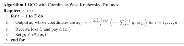
Hence, if we have a 1-dimensional OLO algorithm, we can ${d}$ copies of it, each one fed with the coordinate ${i}$ of the subgradient. In particular, we might think to use the KT algorithm over each coordinate. The pseudo-code of this procedure is in Algorithm 1.

kt_coordinate

The regret bound we get is immediate: We just have to sum the regret over the coordinates.

Theorem 1 With the notation in Algorithm 1, assume that ${\|{\boldsymbol g}_t\|_\infty\leq 1}$ . Then, ${\forall {\boldsymbol u} \in {\mathbb R}^d}$ , the following regret bounds hold

$\displaystyle \sum_{t=1}^T (\ell_t({\boldsymbol x}_t)- \ell_t({\boldsymbol u})) \leq \sum_{i=1}^d |u_i| \sqrt{4 T \ln \left(1+ \frac{\sqrt{2} u_i^2 K T}{\epsilon}\right)} + d \epsilon \leq \|{\boldsymbol u}\|_1 \sqrt{4 T \ln \left(1+ \frac{\sqrt{2} \|{\boldsymbol u}\|_\infty^2 K T}{\epsilon}\right)} + d \epsilon,$

where ${K}$ is a universal constant.

Note that the Theorem above suggests that in high dimensional settings ${\epsilon}$ should be proportional to ${\frac{1}{d}}$ .

2. Parameter-free in Any Norm

The above reductions works only with in a finite dimensional space. Moreover, it gives a dependency on the competitor w.r.t. the ${L_1}$ norm that might be undesirable. So, here we present another simple reduction from 1-dimensional OCO to infinite dimensions.

This reduction requires an unconstrained OCO algorithm for the 1-dimensional case and an algorithm for learning in ${d}$ -dimensional (or infinite dimensional) balls. For the 1-dimensional learner, we could use the KT algorithm, while for learning in ${d}$ -dimensional balls we can use, for example, Online Mirror Descent (OMD). Given these two learners, we decompose the problem of learning a vector ${{\boldsymbol x}_t}$ in the problem of learning a direction and a magnitude. The regret of this procedure turns out to be just the sum of the regret of the two learners.

We can formalize this idea in the following Theorem.

magnitude_direction

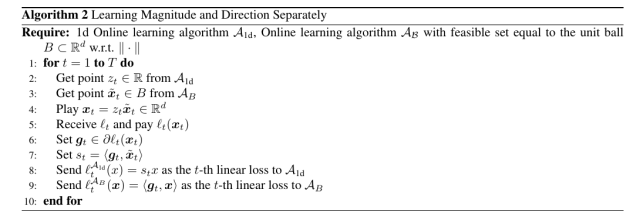
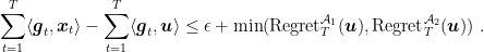
Theorem 2 Denote by ${\text{Regret}^{\mathcal{A}_{B}}_T({\boldsymbol u})}$ the linear regret of algorithm ${\mathcal{A}_{B}}$ for any ${{\boldsymbol u}}$ in the unit ball w.r.t a norm ${\|\cdot\|}$ , and ${\text{Regret}^{\mathcal{A}_{\text{1d}}}_T(u)}$ the linear regret of algorithm ${\mathcal{A}_{\text{1d}}}$ for any competitor ${u \in{\mathbb R}}$ . Then, for any ${{\boldsymbol u}\in {\mathbb R}^d}$ , Algorithm 2 guarantees regret

$\displaystyle \text{Regret}_T({\boldsymbol u}) = \sum_{t=1}^T \ell_t({\boldsymbol x}_t) - \sum_{t=1}^T \ell_t({\boldsymbol u}) \leq \sum_{t=1}^T \langle {\boldsymbol g}_t, {\boldsymbol x}_t -{\boldsymbol u}\rangle = \text{Regret}^{\mathcal{A}_{\text{1d}}}_T(\|{\boldsymbol u}\|) + \|{\boldsymbol u}\| \text{Regret}^{\mathcal{A}_{B}}_T\left(\frac{{\boldsymbol u}}{\|{\boldsymbol u}\|}\right)~.$

Further, the subgradients ${s_t}$ sent to ${\mathcal{A}_{\text{1d}}}$ satisfy ${|s_t|\le \|{\boldsymbol g}_t\|_\star}$ .

Proof: First, observe that ${|s_t|\le \|{\boldsymbol g}_t\|_\star \|\tilde{{\boldsymbol x}}_t\| \le \|{\boldsymbol g}_t\|_\star}$ since ${\|\tilde{{\boldsymbol x}}_t\|\le 1}$ for all ${t}$ . Now, compute:

$\displaystyle \begin{aligned} \text{Regret}_T({\boldsymbol u}) &=\sum_{t=1}^T \ell_t({\boldsymbol x}_t) - \sum_{t=1}^T \ell_t({\boldsymbol u}) \leq \sum_{t=1}^T \langle {\boldsymbol g}_t, {\boldsymbol x}_t - {\boldsymbol u}\rangle = \sum_{t=1}^T \langle {\boldsymbol g}_t, z_t \tilde{{\boldsymbol x}}_t\rangle - \langle {\boldsymbol g}_t, {\boldsymbol u}\rangle\\ &= \underbrace{\sum_{t=1}^T \left(\langle {\boldsymbol g}_t, \tilde{{\boldsymbol x}}_t \rangle z_t - \langle {\boldsymbol g}_t, \tilde{{\boldsymbol x}}_t\rangle \|{\boldsymbol u}\|\right)}_{\text{linear regret of }\mathcal{A}_{\text{1d}}\text{ at } \|{\boldsymbol u}\| \in {\mathbb R}} + \sum_{t=1}^T \left(\langle {\boldsymbol g}_t, \tilde{{\boldsymbol x}}_t \rangle \|{\boldsymbol u}\| - \langle {\boldsymbol g}_t, {\boldsymbol u} \rangle \right)\\ &= \text{Regret}^{\mathcal{A}_{\text{1d}}}_T(\|{\boldsymbol u}\|) + \sum_{t=1}^T \left(\langle {\boldsymbol g}_t, \tilde{{\boldsymbol x}}_t\rangle \|{\boldsymbol u}\| - \langle {\boldsymbol g}_t, {\boldsymbol u}\rangle \right)\\ &= \text{Regret}^{\mathcal{A}_{\text{1d}}}_T(\|{\boldsymbol u}\|) +\|{\boldsymbol u}\| \sum_{t=1}^T \left(\langle {\boldsymbol g}_t, \tilde{{\boldsymbol x}}_t\rangle - \left\langle {\boldsymbol g}_t, \frac{{\boldsymbol u}}{\|{\boldsymbol u}\|}\right\rangle \right)\\ &= \text{Regret}^{\mathcal{A}_{\text{1d}}}_T(\|{\boldsymbol u}\|) + \|{\boldsymbol u}\| \text{Regret}^{\mathcal{A}_{B}}_T\left(\frac{{\boldsymbol u}}{\|{\boldsymbol u}\|}\right)~. \end{aligned}$

$\Box$

Remark 1 Note that the direction vector is not constrained to have norm equal to 1, yet this does not seem to affect the regret equality.

We can instantiate the above theorem using the KT betting algorithm for the 1d learner and OMD for the direction learner. We obtain the following examples.

Example 1 Let ${\mathcal{A}_{B}}$ be OSD with ${V=\{{\boldsymbol x} \in {\mathbb R}^d : \|{\boldsymbol x}\|_2\leq 1\}}$ and learning rate ${\eta_t=\frac{\sqrt{2}D}{2\sqrt{t}}}$ . Let ${\mathcal{A_{\text{1d}}}}$ the KT algorithm for 1-dimensional OCO with ${\epsilon=1}$ . Assume the loss functions are ${1}$ -Lipschitz w.r.t. the ${\|\cdot\|_2}$ . Then, using the construction in Algorithm 2, we have

$\displaystyle \text{Regret}_T({\boldsymbol u}) \leq O\left(\left(\|{\boldsymbol u}\|_2 \sqrt{\ln(\|{\boldsymbol u}\|_2 T+1)} +1\right) \sqrt{T} + 1\right), \ \forall {\boldsymbol u} \in {\mathbb R}^d~.$

Using an online-to-batch conversion, this algorithm is a stochastic gradient descent procedure without learning rates to tune.

To better appreciate this kind of guarantee, let’s take a look at the one of Follow-The-Regularized-Leader (Online Subgradient Descent can be used in unbounded domains only with constant learning rates). With the regularizer ${\psi_t({\boldsymbol x})=\frac{\sqrt{t}}{2\alpha}\|{\boldsymbol x}\|_2}$ and 1-Lipschitz losses we get a regret of

$\displaystyle \text{Regret}_T({\boldsymbol u}) \leq \sqrt{T}\left(\frac{\|{\boldsymbol u}\|^2_2}{2\alpha}+\alpha\right)~.$

So, to get the right dependency on ${\|{\boldsymbol u}\|_2}$ we need to tune ${\alpha}$ , but we saw this is impossible. On the other hand, the regret in Example 1 suffers from a logarithmic factor, that is the price to pay not to have to tune parameters.

In the same way, we can even have a parameter-free regret bound for ${L_p}$ norms.

Example 2 Let ${\mathcal{A}_{B}}$ be OMD with ${V=\{{\boldsymbol x} \in {\mathbb R}^d : \|{\boldsymbol x}\|_p\leq 1\}}$ and learning rate ${\eta_t=\frac{\sqrt{2(p-1)}D}{2\sqrt{t}}}$ . Let ${\mathcal{A_{\text{1d}}}}$ the KT algorithm for 1-dimensional OCO with ${\epsilon=1}$ . Assume the loss functions are ${1}$ -Lipschitz w.r.t. the ${\|\cdot\|_q}$ . Then, using the construction in Algorithm 2, we have

$\displaystyle \text{Regret}_T({\boldsymbol u}) \leq O\left(\left(\|{\boldsymbol u}\|_p \sqrt{\ln(\|{\boldsymbol u}\|_p T+1)} + \frac{\|{\boldsymbol u}\|_p}{\sqrt{p-1}}\right) \sqrt{T} +1\right), \ \forall {\boldsymbol u} \in {\mathbb R}^d~.$

If we want to measure the competitor w.r.t the ${L_1}$ norm, we have to use the same method we saw for OMD: Set ${q=2 \ln d}$ and ${p}$ such that ${1/p+1/q=1}$ . Now, assuming that ${\|{\boldsymbol g}_t\|_\infty\leq 1}$ , we have that ${\|{\boldsymbol g}_t\|_q\leq d^{1/q}}$ . Hence, we have to divide all the losses by ${d^{1/q}}$ and, for all ${{\boldsymbol u} \in {\mathbb R}^d}$ , we obtain

$\displaystyle \begin{aligned} d^{-1/q} \sum_{t=1}^T (\ell_t({\boldsymbol x}_t) - \ell_t({\boldsymbol u})) &\leq O\left(\left(\|{\boldsymbol u}\|_p \sqrt{\ln(\|{\boldsymbol u}\|_p T+1)} + \|{\boldsymbol u}\|_p\sqrt{q-1}\right) \sqrt{T} +1\right) \\ &\leq O\left(\left(\|{\boldsymbol u}\|_1 \sqrt{\ln(\|{\boldsymbol u}\|_1 T+1)} + \|{\boldsymbol u}\|_1\sqrt{\ln d}\right) \sqrt{T} +1\right)~. \end{aligned}$

Note that the regret against ${{\boldsymbol u}=\boldsymbol{0}}$ of the parameter-free construction is constant. It is important to understand that there is nothing special in the origin: We could translate the prediction by any offset and get a guarantee that treats the offset as the point with constant regret. This is shown in the next Proposition.

Proposition 3 Let ${\mathcal{A}}$ an OLO algorithm that predicts ${{\boldsymbol x}_t}$ and guarantees linear regret ${\text{Regret}^{OLO}_T({\boldsymbol u})}$ for any ${{\boldsymbol u} \in {\mathbb R}^d}$ . We have that the regret of the predictions ${\hat{{\boldsymbol x}}_t={\boldsymbol x}_t+{\boldsymbol x}_0}$ for OCO is

$\displaystyle \sum_{t=1}^T \ell_t(\hat{{\boldsymbol x}}_t) - \sum_{t=1}^T \ell_t({\boldsymbol u}) \leq \sum_{t=1}^T \langle {\boldsymbol g}_t, {\boldsymbol x}_t + {\boldsymbol x}_0 - {\boldsymbol u}\rangle = \text{Regret}^{OLO}_T({\boldsymbol u}-{\boldsymbol x}_0)~.$

3. Combining OCO Algorithms

Finally, we now show a useful application of the parameter-free OCO algorithms property to have a constant regret against ${{\boldsymbol u}=\boldsymbol{0}}$ .

Theorem 4 Let ${\mathcal{A}_1}$ and ${\mathcal{A}_2}$ two OLO algorithms that produces the predictions ${{\boldsymbol x}_{t,1}}$ and ${{\boldsymbol x}_{t,2}}$ respectively. Then, predicting with ${{\boldsymbol x}_t={\boldsymbol x}_{t,1}+{\boldsymbol x}_{t,2}}$ , we have for any ${{\boldsymbol u} \in {\mathbb R}^d}$

$\displaystyle \sum_{t=1}^T \langle {\boldsymbol g}_t, {\boldsymbol x}_t\rangle - \sum_{t=1}^T \langle {\boldsymbol g}_t, {\boldsymbol u}\rangle = \min_{{\boldsymbol u}={\boldsymbol u}_1+{\boldsymbol u}_2} \ \text{Regret}^{\mathcal{A}_1}_T({\boldsymbol u}_1) + \text{Regret}^{\mathcal{A}_2}_T({\boldsymbol u}_2)~.$

Moreover, if both algorithm guarantee a constant regret of ${\epsilon}$ against ${{\boldsymbol u}=\boldsymbol{0}}$ , we have for any ${{\boldsymbol u} \in {\mathbb R}^d}$

$\displaystyle \sum_{t=1}^T \langle {\boldsymbol g}_t, {\boldsymbol x}_t\rangle - \sum_{t=1}^T \langle {\boldsymbol g}_t, {\boldsymbol u}\rangle \leq \epsilon + \min(\text{Regret}^{\mathcal{A}_1}_T({\boldsymbol u}), \text{Regret}^{\mathcal{A}_2}_T({\boldsymbol u}))~.$

Proof: Set ${{\boldsymbol u}_1+{\boldsymbol u}_2={\boldsymbol u}}$ . Then,

$\displaystyle \sum_{t=1}^T \langle {\boldsymbol g}_t, {\boldsymbol x}_t\rangle - \sum_{t=1}^T \langle {\boldsymbol g}_t, {\boldsymbol u}\rangle =\sum_{t=1}^T \langle {\boldsymbol g}_t, {\boldsymbol x}_{t,1}\rangle - \sum_{t=1}^T \langle {\boldsymbol g}_t, {\boldsymbol u}_1\rangle +\sum_{t=1}^T \langle {\boldsymbol g}_t, {\boldsymbol x}_{t,2}\rangle - \sum_{t=1}^T \langle {\boldsymbol g}_t, {\boldsymbol u}_2\rangle~.$

$\Box$

In words, the above theorem allows us to combine online learning algorithm. If the algorithms we combine have constant regret against the null competitor, then we always get the best of the two guarantees.

Example 3 We can combine two parameter-free OCO algorithms, one that gives a bound that depends on the ${L_2}$ norm of the competitor and subgradients and another one specialized to the ${L_1/L_\infty}$ norm of competitor/subgradients. The above theorem assures us that we will also get the best guarantee between the two, paying only a constant factor in the regret.

Of course, upper bounding the OCO regret with the linear regret, the above theorem also upper bounds the OCO regret.

4. History Bits

The approach of using a coordinate-wise version of the coin-betting algorithm was proposed in the first paper on parameter-free OLO in (M. Streeter and B. McMahan, 2012). Recently, the same approach with a special coin-betting algorithm was also used for optimization of deep neural networks (Orabona, F. and Tommasi, T., 2017). Theorem 2 is from (A. Cutkosky and F. Orabona, 2018). Note that the original theorem is more general because it works even in Banach spaces. The idea of combining two parameter-free OLO algorithms to obtain the best of the two guarantees is from (A. Cutkosky, 2019).

(Orabona, F. and Pal, D., 2016) proposed a different way to transform a coin-betting algorithm into an OCO algorithm that works in ${{\mathbb R}^d}$ or even in Hilbert spaces. However, that approach seems to work on for the ${L_2}$ norm and it is not a black-box reduction. That said, the reduction in (Orabona, F. and Pal, D., 2016) seems to have a better empirical performance compared to the one in Theorem 2.

There are also reductions that allow to transform an unconstrained OCO learner into a constrained one (A. Cutkosky and F. Orabona, 2018). They work constructing a Lipschitz barrier function on the domain and passing to the algorithm the original subgradients plus the subgradients of the barrier function.

5. Exercises

Exercise 1 Prove that ${\ell_t(x)=-\ln(1+ z_t\, x)}$ with ${V=\{x \in {\mathbb R}: |x|\leq 1/2\}}$ and ${|z_t|\leq 1, \ t=1,\dots,T}$ are exp-concave. Then, using the Online Newton Step Algorithm, give an algorithm and a regret bound for a game with these losses. Finally, show a wealth guarantee of the corresponding coin-betting strategy.

3 Comments

Pingback: Parameter-free Online Learning III: from Coins to Experts – Parameter-free Learning and Optimization Algorithms
Nicolò says:

December 1, 2019 at 7:13 PM

Hi Francesco, very nice post!
Few comments: in Algorithm 2 line 3 I think $\tilde{x}$ should be in B, not S. Also it’s not totally clear what losses we feed to the 2 algorithms, but if I understood well they should be $\ell_t^{\mathcal{A}_{1d}} (z_t) $ for the KT algo and $ \ell_t^{\mathcal{A}_B} (\tilde{x}_t) $ to MD, right?
Also, some typos: in the second line of the proof of Theorem 2, the subscript t is missing from $ \tilde{x} $, while in the second bound of Theorem 4, the min is between R_T(u) (instead of R_T(u_1)) and R_T(u_2).

LikeLike

1. bremen79 says:
  
  December 3, 2019 at 5:31 PM
  
  Fixed all the typos, thanks!
  Regarding passing the losses in Algorithm 2: I am not sure I understand your concern, here we pass the entire loss to the direction and magnitude learners, and they will use them as they like. I don’t just pass the value of the losses on their predictions, right?
  
  LikeLike
  
  1. Nicolò says:
    
    December 4, 2019 at 12:26 PM
    
    Yes, I totally agree. I got confused by the notation somehow.
    
    Thanks
    
    LikeLike