A Simple Proof for Optimistic OMD

While preparing the post on faster rates for saddle-point optimization with optimistic Online Convex Optimization algorithms, I realized I never explained Optimistic Online Mirror Descent (OMD). So, here it is: Optimistic OMD!

The post will be short: the algorithm is straightforward, especially after knowing Optimistic Follow-The-Regularized-Leader (FTRL), and the proof is the simplest one I know. Yet, there are few interesting bits that one can extract from this short proof.

1. Optimistic OMD

I have already discussed the Optimistic version of FTRL and show how the proof is immediate once we change the regularizers. By immediate, I mean that it is just the FTRL regret equality and a telescopic sum over the hints. Here, I’ll show that a regret bound for Optimistic OMD can be proven in the exact same way.

I always found previous proofs of optimistic OMD unnecessarily complex. Instead, here we show that the proof is just the usual OMD proof applied to a different sequence of subgradients and a telescopic sum: easy peasy! I want to stress that this is not a “trick”, but the very essence of the Optimistic OMD algorithm.

First, let’s introduce the Optimistic OMD algorithm, see Algorithm 1. Here, at round ${t}$ the algorithm receives a hint ${\tilde{{\boldsymbol g}}_{t+1}}$ on the next subgradient ${{\boldsymbol g}_{t+1}}$ and uses it to construct the update. At the same time, you have to remove the hint you used at the previous time step, ${\tilde{{\boldsymbol g}}_{t}}$ . (Note that this is the more recent one-update-per-step variant of Optimistic OMD, rather than the original two-updates-per-step Optimistic OMD, see the History Bits.)

optimistic_omd

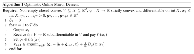
To gain some intuition on why this update makes sense, consider the case that ${\psi({\boldsymbol x})=\frac{1}{2}\|{\boldsymbol x}\|_2^2}$ , ${\eta_t=\eta}$ , and ${V={\mathbb R}^d}$ . In this case, ${{\boldsymbol x}_{t+1} = {\boldsymbol x}_{t} + \eta \tilde{{\boldsymbol g}}_{t} - \eta {\boldsymbol g}_t - \eta \tilde{{\boldsymbol g}}_{t+1}}$ . Unrolling the update, we get ${{\boldsymbol x}_{t+1} = {\boldsymbol x}_1 - \eta (\tilde{{\boldsymbol g}}_{t+1}+\sum_{i=1}^t {\boldsymbol g}_i)}$ . Without hints, that is in plain OMD, under the same assumptions the unrolled update would be ${{\boldsymbol x}_{t+1} = {\boldsymbol x}_1 - \eta \sum_{i=1}^t {\boldsymbol g}_i}$ and ${{\boldsymbol x}_{t+2} = {\boldsymbol x}_1 - \eta \sum_{i=1}^{t+1} {\boldsymbol g}_i}$ . Hence, ${\tilde{{\boldsymbol g}}_{t+1}}$ acts as a proxy for the next (unknown) subgradient ${{\boldsymbol g}_t}$ .

Note that one might be tempted to multiply ${\tilde{{\boldsymbol g}}_t}$ by ${\eta_{t-1}}$ , because in the previous iteration we used the learning rate ${\eta_{t-1}}$ . However, the online learning proof reveals that the correct way to see the update is to think the learning rate as attached to the Bregman divergence rather than to the subgradients. (Things might be different in the batch and stochastic setting, where the best proofs deal with the learning rates in a slightly different way.)

One might also be tempted to find a way to study this algorithm with a special proof. However, the one-step lemma we proved for OMD is essentially tight: we only used two inequalities, one to deal with the set ${V}$ and the other one to linearize the losses. But, but both steps can be made tight, considering ${V={\mathbb R}^d}$ and linear losses. Hence, if the update is just OMD with a different sequence of subgradients, the proof must follow from the one of OMD with a different set of subgradients. This is a general rule: If we have a theorem based on a tight inequality, any other proof of the same theorem, no matter how complex, must be looser or in the best case equivalent. On the other hand, some (fake) complexity might help you with some reviewers, but this is another story… 😉

Theorem 1. Let ${B_\psi}$ the Bregman divergence w.r.t. ${\psi: X \rightarrow {\mathbb R}}$ and assume ${\psi}$ to be proper, closed, and ${\lambda}$ -strongly convex with respect to ${\|\cdot\|}$ in ${V}$ . Let ${V \subseteq X}$ a non-empty closed convex set. With the notation in Algorithm 1, assume ${{\boldsymbol x}_{t+1}}$ exists, and it is in ${\mathop{\mathrm{int}} X}$ .

Assume ${\eta_{t+1}\leq \eta_{t}, \ t=1, \dots, T}$ . Then, and ${\forall {\boldsymbol u} \in V}$ , the following regret bounds hold

$\displaystyle \begin{aligned} \sum_{t=1}^T (\ell_t({\boldsymbol x}_t)- \ell_t({\boldsymbol u})) &\leq \max_{1\leq t \leq T} \frac{B_\psi({\boldsymbol u};{\boldsymbol x}_t)}{\eta_{T}} + \sum_{t=1}^T \left(\langle {\boldsymbol g}_t-\tilde{{\boldsymbol g}}_t,{\boldsymbol x}_{t}-{\boldsymbol x}_{t+1}\rangle- \frac{1}{\eta_t} B_\psi({\boldsymbol x}_{t+1};{\boldsymbol x}_t)\right) \\ &\leq \max_{1\leq t \leq T} \frac{B_\psi({\boldsymbol u};{\boldsymbol x}_t)}{\eta_{T}} + \frac{1}{2\lambda}\sum_{t=1}^T \eta_t \|{\boldsymbol g}_t-\tilde{{\boldsymbol g}}_t\|^2_\star~. \end{aligned}$

Moreover, if ${\eta_t}$ is constant, i.e., ${\eta_t=\eta \ \forall t=1,\cdots,T}$ , we have

$\displaystyle \begin{aligned} \sum_{t=1}^T (\ell_t({\boldsymbol x}_t)- \ell_t({\boldsymbol u})) &\leq \frac{B_\psi({\boldsymbol u};{\boldsymbol x}_1)}{\eta} + \sum_{t=1}^T \left(\langle {\boldsymbol g}_t-\tilde{{\boldsymbol g}}_t,{\boldsymbol x}_{t}-{\boldsymbol x}_{t+1}\rangle- \frac{1}{\eta} B_\psi({\boldsymbol x}_{t+1};{\boldsymbol x}_t)\right)\\ &\leq \frac{B_\psi({\boldsymbol u};{\boldsymbol x}_1)}{\eta} + \frac{\eta}{2\lambda}\sum_{t=1}^T \|{\boldsymbol g}_t-\tilde{{\boldsymbol g}}_t\|^2_\star~. \end{aligned}$

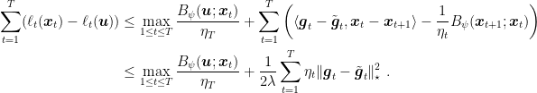
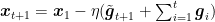
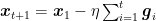
Proof: The proof closely follows the one of Lemma 4 in the OMD proof with ${{\boldsymbol g}_t \rightarrow {\boldsymbol g}_t - \tilde{{\boldsymbol g}}_t + \tilde{{\boldsymbol g}}_{t+1}}$ , so we only show the different steps. First of all, changing the sequence of subgradients, we immediately have

$\displaystyle \langle {\boldsymbol g}_t - \tilde{{\boldsymbol g}}_t + \tilde{{\boldsymbol g}}_{t+1}, {\boldsymbol x}_t - {\boldsymbol u}\rangle \leq \frac{1}{\eta_t}\left(B_\psi({\boldsymbol u};{\boldsymbol x}_t) - B_\psi({\boldsymbol u};{\boldsymbol x}_{t+1}) - B_\psi({\boldsymbol x}_{t+1};{\boldsymbol x}_t)\right) + \langle {\boldsymbol g}_t - \tilde{{\boldsymbol g}}_t + \tilde{{\boldsymbol g}}_{t+1}, {\boldsymbol x}_t - {\boldsymbol x}_{t+1} \rangle~.$

Summing over ${t=1,\dots,T}$ the l.h.s., we obtain

$\displaystyle \begin{aligned} \sum_{t=1}^T \langle {\boldsymbol g}_t - \tilde{{\boldsymbol g}}_t + \tilde{{\boldsymbol g}}_{t+1}, {\boldsymbol x}_t - {\boldsymbol u}\rangle &= \sum_{t=1}^T \langle {\boldsymbol g}_t, {\boldsymbol x}_t - {\boldsymbol u}\rangle + \sum_{t=1}^T \langle \tilde{{\boldsymbol g}}_{t+1} -\tilde{{\boldsymbol g}}_t, {\boldsymbol x}_t-{\boldsymbol u}\rangle \\ &= \sum_{t=1}^T \langle {\boldsymbol g}_t, {\boldsymbol x}_t - {\boldsymbol u}\rangle + \langle \tilde{{\boldsymbol g}}_{1} - \tilde{{\boldsymbol g}}_{T+1}, {\boldsymbol u}\rangle + \sum_{t=1}^T \langle \tilde{{\boldsymbol g}}_{t+1} - \tilde{{\boldsymbol g}}_t, {\boldsymbol x}_t\rangle~. \end{aligned}$

Summing the last terms on the r.h.s., we have that

$\displaystyle \begin{aligned} \sum_{t=1}^T \langle {\boldsymbol g}_t - \tilde{{\boldsymbol g}}_t + \tilde{{\boldsymbol g}}_{t+1}, {\boldsymbol x}_t - {\boldsymbol x}_{t+1} \rangle &= \sum_{t=1}^T \langle {\boldsymbol g}_t-\tilde{{\boldsymbol g}}_{t}, {\boldsymbol x}_t - {\boldsymbol x}_{t+1} \rangle + \sum_{t=1}^T \langle \tilde{{\boldsymbol g}}_{t+1}, {\boldsymbol x}_t - {\boldsymbol x}_{t+1} \rangle~. \end{aligned}$

Finally, observe that

$\displaystyle \sum_{t=1}^T \langle \tilde{{\boldsymbol g}}_{t+1} - \tilde{{\boldsymbol g}}_t, {\boldsymbol x}_t\rangle - \sum_{t=1}^T \langle \tilde{{\boldsymbol g}}_{t+1}, {\boldsymbol x}_t - {\boldsymbol x}_{t+1} \rangle = \sum_{t=1}^T (\langle \tilde{{\boldsymbol g}}_{t+1},{\boldsymbol x}_{t+1}\rangle -\langle \tilde{{\boldsymbol g}}_t,{\boldsymbol x}_t\rangle) = \langle \tilde{{\boldsymbol g}}_{T+1},{\boldsymbol x}_{T+1}\rangle - \langle \tilde{{\boldsymbol g}}_1,{\boldsymbol x}_1\rangle~.$

Given that loss on the rounds ${t=1,\dots,T}$ does not depend on ${\tilde{{\boldsymbol g}}_{T+1}}$ we can safely set it to ${\boldsymbol{0}}$ . Putting all together, we have the stated bounds.

To obtain the second inequalities, we use the strong convexity of ${\psi}$ as in the proof of OMD. $\Box$

These regret bounds are essentially the same of the ones of Optimistic FTRL, minus the intrinsic differences between FTRL and OMD. In particular, the constant factors are also the same. Hence, similar results to the ones that we proved for Optimistic FTRL can be proved for Optimistic OMD.

As said above, we will use this result to show how to accelerate the optimization of smooth saddle-point problems.

2. History Bits

The original Optimistic OMD was proposed in Rakhlin and Sridharan (2013) with two-updates-per-step. Later, Joulani et al. (2017) showed that the same bounds could be obtained with a simpler one-update-per-step version of Optimistic OMD, that is the version I describe here. The proof I present here is based on the one I proposed for Optimistic FTRL.

Pingback: Saddle-Point Optimization With Optimism – Parameter-free Learning and Optimization Algorithms

Share this:

Like this:

Related

Leave a Reply Cancel reply