Saddle-Point Optimization With Optimism

In the latest posts, we saw that it is possible to solve convex/concave saddle-point optimization problems using two online convex optimization algorithms playing against each other. We obtained a rate of convergence for the duality gap of ${O(1/\sqrt{T})}$ . This time we show that if the function is smooth we can achieve a faster rate using optimistic algorithms.

1. Faster Rates Through Optimism

Assume that ${f:X\times Y \rightarrow {\mathbb R}}$ is smooth in an open interval containing its domain, in the sense that for any ${{\boldsymbol x},{\boldsymbol x}'\in X}$ and ${{\boldsymbol y},{\boldsymbol y}' \in Y}$ , we have

$\displaystyle \begin{aligned} \|\nabla_{{\boldsymbol x}} f({\boldsymbol x},{\boldsymbol y})-\nabla_{{\boldsymbol x}} f({\boldsymbol x}',{\boldsymbol y})\|_{X,\star} &\leq L_{XX} \|{\boldsymbol x}-{\boldsymbol x}'\|_{X} & (1) \\ \|\nabla_{{\boldsymbol x}} f({\boldsymbol x},{\boldsymbol y})-\nabla_{{\boldsymbol x}} f({\boldsymbol x},{\boldsymbol y}')\|_{X,\star} &\leq L_{XY} \|{\boldsymbol y}-{\boldsymbol y}'\|_{Y} & (2) \\ \|\nabla_{{\boldsymbol y}} f({\boldsymbol x},{\boldsymbol y})-\nabla_{{\boldsymbol y}} f({\boldsymbol x}',{\boldsymbol y})\|_{Y,\star} &\leq L_{XY} \|{\boldsymbol x}-{\boldsymbol x}'\|_{X} & (3) \\ \|\nabla_{{\boldsymbol y}} f({\boldsymbol x},{\boldsymbol y})-\nabla_{{\boldsymbol y}} f({\boldsymbol x},{\boldsymbol y}')\|_{Y,\star} &\leq L_{YY} \|{\boldsymbol y}-{\boldsymbol y}'\|_{Y}, & (4) \\\end{aligned}$

where ${\nabla_{{\boldsymbol x}}}$ and ${\nabla_{{\boldsymbol y}}}$ denote the gradients with respect to the first and second variable respectively, and we have denoted by ${\|\cdot\|_{X}}$ and ${\|\cdot\|_Y}$ the norms in ${X}$ and ${Y}$ respectively, while the norms with the ${\star}$ are their duals.

Remark 1. At this point, one might be tempted to consider the maximum between the three quantities “to simplify the math”, but the units are different!

Let’s use again two online algorithms to solve the saddle-point problem ${\min_{{\boldsymbol x} \in X} \max_{{\boldsymbol y} \in Y} \ f({\boldsymbol x},{\boldsymbol y})}$ . However, instead of using two standard no-regret algorithms, we will use two optimistic ones. Optimistic online algorithms use a hint on the next subgradient. We will use the same strategy and proof of the algorithm we saw for gradual variations, that is we will use the previous observed gradient as a prediction for the next one.

For example, use two Optimistic FTRL algorithms with fixed strongly convex regularizers and hint at time ${t}$ constructed using the previous observed gradient: ${\tilde{\ell}_t({\boldsymbol x})=\langle {\boldsymbol g}_{t-1}, {\boldsymbol x}\rangle}$ where we set ${{\boldsymbol g}_0=0}$ . We now show that these hints allow to cancel out terms when we consider the sum of the regrets and obtain a faster rate of ${O(1/T)}$ rather than just ${O(1/\sqrt{T})}$ .

From the regret of Optimistic FTRL, for the ${X}$ -player we have

$\displaystyle \sum_{t=1}^T (\ell_t({\boldsymbol x}_t)-\ell({\boldsymbol u})) \leq \psi_X({\boldsymbol u}) + \sum_{t=1}^T \left(\langle {\boldsymbol g}_{X,t} - {\boldsymbol g}_{X,t-1}, {\boldsymbol x}_t - {\boldsymbol x}_{t+1}\rangle -\frac{\lambda_X}{2} \|{\boldsymbol x}_t-{\boldsymbol x}_{t+1}\|^2_X\right), \ \forall {\boldsymbol u} \in X~.$

From the Fenchel-Young inequality, we have ${\langle {\boldsymbol g}_{X,t} - {\boldsymbol g}_{X,t-1}, {\boldsymbol x}_t - {\boldsymbol x}_{t+1}\rangle\leq \frac{\lambda_X}{4}\|{\boldsymbol x}_t - {\boldsymbol x}_{t+1} \|^2_X+ \frac{1}{\lambda_X} \|{\boldsymbol g}_{X,t} - {\boldsymbol g}_{X,t-1}\|^2_{X,\star}}$ . Putting all together, we have

$\displaystyle \sum_{t=1}^T (\ell_t({\boldsymbol x}_t)-\ell({\boldsymbol u})) \leq \psi_X({\boldsymbol u}) +\sum_{t=1}^T \left(\frac{1}{\lambda_X}\|{\boldsymbol g}_{X,t} - {\boldsymbol g}_{X,t-1}\|^2_{X,\star} - \frac{\lambda_X}{4} \|{\boldsymbol x}_t-{\boldsymbol x}_{t+1}\|^2_X\right), \ \forall {\boldsymbol u} \in X~.$

Note that there are multiple choices of the coefficient in the Fenchel-Young inequality, but without additional information all choices are equally good.

Now, using the smoothness assumption, for ${t\geq 2}$ we have

$\displaystyle \begin{aligned} \|{\boldsymbol g}_{X,t} - {\boldsymbol g}_{X,t-1}\|^2_{X,\star} &= \|\nabla_{{\boldsymbol x}} f({\boldsymbol x}_t,{\boldsymbol y}_t) - \nabla_{{\boldsymbol x}} f({\boldsymbol x}_{t-1}, {\boldsymbol y}_{t-1})\|^2_{X,\star} \\ &\leq \left(\|\nabla_{{\boldsymbol x}} f({\boldsymbol x}_t,{\boldsymbol y}_t) - \nabla_{{\boldsymbol x}} f({\boldsymbol x}_{t-1}, {\boldsymbol y}_{t})\|_{X,\star} + \|\nabla_{{\boldsymbol x}} f({\boldsymbol x}_{t-1},{\boldsymbol y}_t) - \nabla_{{\boldsymbol x}} f({\boldsymbol x}_{t-1}, {\boldsymbol y}_{t-1})\|_{X,\star}\right)^2 \\ &\leq 2L_{XX}^2 \|{\boldsymbol x}_{t-1}-{\boldsymbol x}_{t}\|^2_X + 2L^2_{XY} \|{\boldsymbol y}_{t-1} - {\boldsymbol y}_{t}\|^2_Y~. \end{aligned}$

We can proceed in the exact same way for the ${Y}$ -player too.

Summing the regret of the two algorithms, we have

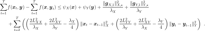
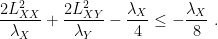
$\displaystyle \begin{aligned} \sum_{t=1}^T &f({\boldsymbol x}_t,{\boldsymbol y}) - \sum_{t=1}^T f({\boldsymbol x},{\boldsymbol y}_t) \leq \psi_X({\boldsymbol x}) + \psi_Y({\boldsymbol y}) + \frac{\|{\boldsymbol g}_{X,1}\|^2_{X,\star}}{\lambda_X}+\frac{\|{\boldsymbol g}_{Y,1}\|^2_{Y,\star}}{\lambda_Y}\\ &+ \sum_{t=2}^T \left(\left(\frac{2L_{XX}^2}{\lambda_X}+\frac{2L^2_{XY}}{\lambda_Y}-\frac{\lambda_X}{4}\right) \|{\boldsymbol x}_t-{\boldsymbol x}_{t-1}\|^2_X + \left(\frac{2L^2_{YY}}{\lambda_Y}+\frac{2L^2_{XY}}{\lambda_X}-\frac{\lambda_Y}{4}\right) \|{\boldsymbol y}_t-{\boldsymbol y}_{t-1}\|^2_Y\right)~. \end{aligned}$

Choosing ${\lambda_X \geq 2 \sqrt{2} (L_{XX}+L_{XY} \alpha)}$ and ${\lambda_Y\geq 2 \sqrt{2}(L_{YY}+L_{XY}/\alpha)}$ for any ${\alpha>0}$ kills all the terms in the sum. In fact, we have

$\displaystyle \frac{2L_{XX}^2}{\lambda_X}+\frac{2L^2_{XY}}{\lambda_Y} \leq \frac{2L_{XX}^2}{2\sqrt{2} L_{XX}}+\frac{2L^2_{XY} \alpha}{2 \sqrt{2} L_{XY}} \leq \frac{\lambda_X}{4},$

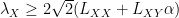
and similarly for the other term. One might wonder why we need to introduce ${\alpha}$ and if it can be just set to 1. However, ${\alpha}$ has units and it allows the sum of the smoothness coefficients, so it is better to keep it around to remember it.

Assuming that the regularizers are bounded over ${X}$ and ${Y}$ and using the usual online-to-batch conversion, we have that the duality gap evaluated at the pair ${\left(\frac{1}{T}\sum_{t=1}^T {\boldsymbol x}_t, \frac{1}{T}\sum_{t=1}^T {\boldsymbol y}_t\right)}$ goes to zero as ${O(1/T)}$ when ${T\rightarrow\infty}$ .

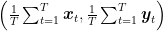
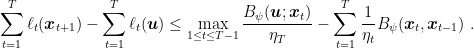
Overall, we can state the following theorem.

Theorem 1. With the notation in Algorithm 1, let ${f:X\times Y\rightarrow {\mathbb R}}$ convex in the first argument and concave in the second, satisfying assumptions (1)–(4). For a fixed ${\alpha>0}$ , let ${\lambda_X \geq 2 \sqrt{2} (L_{XX}+L_{XY} \alpha)}$ and ${\lambda_Y\geq 2 \sqrt{2}(L_{YY}+L_{XY}/\alpha)}$ . Let ${\psi_X:X\rightarrow{\mathbb R}}$ be ${\lambda_X}$ -strongly convex w.r.t. ${\|\cdot\|_X}$ and ${\psi_Y:Y\rightarrow{\mathbb R}}$ be ${\lambda_Y}$ -strongly convex w.r.t. ${\|\cdot\|_Y}$ . Assume ${\arg\max_{{\boldsymbol y}\in Y}f(\bar{{\boldsymbol x}}_T,{\boldsymbol y})}$ and ${\arg\min_{{\boldsymbol x}\in X}f({\boldsymbol x},\bar{{\boldsymbol y}}_T)}$ non-empty. Then, we have

$\displaystyle \max_{{\boldsymbol y}\in Y} f(\bar{{\boldsymbol x}}_T, {\boldsymbol y}) - \min_{{\boldsymbol x}\in X} f({\boldsymbol x},\bar{{\boldsymbol y}}_T) \leq \frac{\psi_X({\boldsymbol x}'_T)-\psi_X({\boldsymbol x}_1)+\psi_Y({\boldsymbol y}'_T)-\psi_Y({\boldsymbol y}_1)+\frac{\|{\boldsymbol g}_{X,1}\|^2_{X,\star}}{\lambda_X}+\frac{\|{\boldsymbol g}_{Y,1}\|^2_{Y,\star}}{\lambda_Y}}{T},$

for any ${{\boldsymbol x}_T'\in\arg\min_{{\boldsymbol x}\in X}f({\boldsymbol x},\bar{{\boldsymbol y}}_T)}$ and ${{\boldsymbol y}_T'\in\arg\max_{{\boldsymbol y}\in Y}f(\bar{{\boldsymbol x}}_T,{\boldsymbol y})}$ .

Looking back at the proof of the algorithm, we have a faster convergence because regret of one player depends on the “stability” of the other player, measured by the terms ${\|{\boldsymbol x}_t- {\boldsymbol x}_{t-1}\|_X^2}$ and ${\|{\boldsymbol y}_t- {\boldsymbol y}_{t-1}\|_Y^2}$ . Hence, we have a sort of “stabilization loop” in which the stability of one algorithm makes the other more stable, that in turn stabilizes the first one even more. Indeed, we can also show that the regret of the two algorithms is not growing over time. Note that such result cannot be obtained just looking at the fact that the sum of the regret does not grow over time.

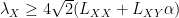
In fact, setting for example ${\lambda_X \geq 4 \sqrt{2} (L_{XX}+L_{XY} \alpha)}$ and ${\lambda_Y\geq 4 \sqrt{2}(L_{YY}+L_{XY}/\alpha)}$ , we have that

$\displaystyle \frac{2L^2_{YY}}{\lambda_Y}+\frac{2L^2_{XY}}{\lambda_X}-\frac{\lambda_Y}{4}\leq -\frac{\lambda_Y}{8}$

and

$\displaystyle \frac{2L_{XX}^2}{\lambda_X}+\frac{2L^2_{XY}}{\lambda_Y}-\frac{\lambda_X}{4} \leq -\frac{\lambda_X}{8}~.$

Hence, using the fact that the existence of a saddle-point ${({\boldsymbol x}^\star, {\boldsymbol y}^\star)}$ guarantee that ${f({\boldsymbol x}_t,{\boldsymbol y}^\star) - f({\boldsymbol x}^\star,{\boldsymbol y}_t)\geq 0}$ , we have

$\displaystyle \label{eq:oftrl_minmax_bounded_sum} \sum_{t=2}^T\left(\frac{\lambda_X}{8} \|{\boldsymbol x}_t-{\boldsymbol x}_{t-1}\|^2_X + \frac{\lambda_Y}{8} \|{\boldsymbol y}_t-{\boldsymbol y}_{t-1}\|^2_Y\right) \leq \psi_X({\boldsymbol x}^\star)-\psi_X({\boldsymbol x}_1)+\psi_Y({\boldsymbol y}^\star)-\psi_Y({\boldsymbol y}_1)+\frac{\|{\boldsymbol g}_{X,1}\|^2_{X,\star}}{\lambda_X}+\frac{\|{\boldsymbol g}_{Y,1}\|^2_{Y,\star}}{\lambda_Y}~. \ \ \ \ \ (5)$

Plugging this guarantee back in the regret of each algorithm, we have that their regret is bounded and independent of ${T}$ . From (5), we also have that ${\|{\boldsymbol x}_t-{\boldsymbol x}_{t-1}\|^2_X}$ and ${\|{\boldsymbol y}_t-{\boldsymbol y}_{t-1}\|^2_Y}$ converge 0. Hence, the algorithms are getting more and more stable over time, even if they use constant regularizers.

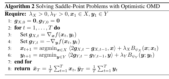
Version with Optimistic OMD The exact same reasoning holds for Optimistic OMD, because the key terms of its regret bound are exactly the same of the one of Optimistic FTRL. To better show this fact, we also instantiate the Optimistic OMD with stepsizes equal to ${\frac{1}{\lambda_X}}$ and ${\frac{1}{\lambda_Y}}$ for ${X}$ -player and ${Y}$ -player respectively. Following the same reasoning above and the regret bound of Optimistic OMD, we obtain the following theorem.

Theorem 2. With the notation in Algorithm 1, let ${f:X\times Y\rightarrow {\mathbb R}}$ convex in the first argument and concave in the second, satisfying assumptions (1)–(4). For a fixed ${\alpha>0}$ , let ${\lambda_X \geq 2 \sqrt{2} (L_{XX}+L_{XY} \alpha)}$ and ${\lambda_Y\geq 2 \sqrt{2}(L_{YY}+L_{XY}/\alpha)}$ . Let ${\psi_X:X\rightarrow{\mathbb R}}$ be ${1}$ -strongly convex w.r.t. ${\|\cdot\|_X}$ and ${\psi_Y:Y\rightarrow{\mathbb R}}$ be ${1}$ -strongly convex w.r.t. ${\|\cdot\|_Y}$ . Assume ${\arg\max_{{\boldsymbol y}\in Y}f(\bar{{\boldsymbol x}}_T,{\boldsymbol y})}$ and ${\arg\min_{{\boldsymbol x}\in X}f({\boldsymbol x},\bar{{\boldsymbol y}}_T)}$ non-empty. Then, we have

$\displaystyle \max_{{\boldsymbol y}\in Y} f(\bar{{\boldsymbol x}}_T, {\boldsymbol y}) - \min_{{\boldsymbol x}\in X} f({\boldsymbol x},\bar{{\boldsymbol y}}_T) \leq \frac{B_{\psi_X}({\boldsymbol x}'_T;{\boldsymbol x}_1)+B_{\psi_Y}({\boldsymbol y}'_T;{\boldsymbol y}_1)+\frac{\|{\boldsymbol g}_{X,1}\|^2_{X,\star}}{\lambda_X}+\frac{\|{\boldsymbol g}_{Y,1}\|^2_{Y,\star}}{\lambda_Y}}{T},$

for any ${{\boldsymbol x}_T'\in\arg\min_{{\boldsymbol x}\in X}f({\boldsymbol x},\bar{{\boldsymbol y}}_T)}$ and ${{\boldsymbol y}_T'\in\arg\max_{{\boldsymbol y}\in Y}f(\bar{{\boldsymbol x}}_T,{\boldsymbol y})}$ .

Example 1. Consider the bilinear saddle-point problem

$\displaystyle \min_{{\boldsymbol x} \in X} \max_{{\boldsymbol y} \in Y} \ {\boldsymbol x}^\top A {\boldsymbol y}~.$

In this case, we have that ${\nabla_{{\boldsymbol x}} f({\boldsymbol x},{\boldsymbol y})=A {\boldsymbol y}}$ , ${\nabla_{{\boldsymbol y}} f({\boldsymbol x},{\boldsymbol y})= A^\top {\boldsymbol x}}$ , ${L_{XX}=0}$ , ${L_{YY}=0}$ , and ${L_{XY}=\|A\|_\text{op}}$ where ${\|\cdot\|_\text{op}}$ is the operator norm of the matrix ${A}$ . The specific shape of the operator norm depends on the norms we use on ${X}$ and ${Y}$ . For example, we choose the Euclidean norm on both ${X}$ and ${Y}$ , the operator norm of ${A}$ is the largest singular value of ${A}$ . On the other hand, if ${X=\Delta^{n-1}}$ and ${\Delta^{m-1}}$ as in the two-person zero-sum games, then the operator norm of a matrix ${A}$ is the maximum absolute value of the entries of ${A}$ .

2. Prescient Online Mirror Descent and Be-The-Regularized-Leader

The above result is interesting from a game-theoretic point of view, because it shows that two player can converge to an equilibrium without any “communication”, if instead we only care about converging to the saddle-point, we can easily do better. In fact, we can use the fact that it is fine if one of the two players “cheats” by looking at the loss at the beginning of each round, making its regret non-positive.

For example, we saw the use of Best Response. However, Best Response only guarantees non-positive regret, while for the optimistic proof above we need some specific negative terms. This is not only an artifact of the proof: Best Response is very unstable and it would ruin the “stabilization loop” we have discussed above. 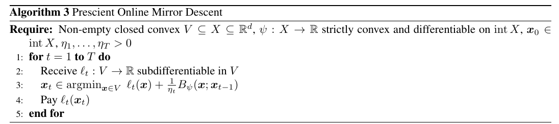It turns out there is an alternative: Prescient Online Mirror Descent, that predicts in each round with ${{\boldsymbol x}_t \in \mathop{\mathrm{argmin}}_{{\boldsymbol x} \in V} \ \ell_t({\boldsymbol x}) + \frac{1}{\eta_t}B_\psi({\boldsymbol x};{\boldsymbol x}_{t-1})}$ . We can intepret it as a conservative version of Best Response that trade-offs the best response with the distance from its previous prediction.

Theorem 3. Let ${\psi: X \rightarrow {\mathbb R}}$ differentiable in ${\mathop{\mathrm{int}} X}$ , closed, and strictly convex. Let ${V \subseteq X}$ a non-empty closed convex set. Assume ${{\boldsymbol x}_t \in \mathop{\mathrm{int}} X}$ , ${\ell_t}$ subdifferentiable in ${V}$ , and ${\eta_{t+1}\leq \eta_{t}}$ , for ${t=1, \dots, T}$ . Then, ${\forall {\boldsymbol u} \in V}$ , the following inequality holds

$\displaystyle \sum_{t=1}^T \ell_t({\boldsymbol x}_{t+1}) - \sum_{t=1}^T \ell_t({\boldsymbol u}) \leq \max_{1\leq t \leq T-1} \frac{B_\psi({\boldsymbol u};{\boldsymbol x}_t)}{\eta_{T}} - \sum_{t=1}^T \frac{1}{\eta_t} B_\psi({\boldsymbol x}_{t}, {\boldsymbol x}_{t-1} ) ~.$

Moreover, if ${\eta_t}$ is constant, i.e., ${\eta_t=\eta \ \forall t=1,\cdots,T}$ , we have

$\displaystyle \sum_{t=1}^T (\ell_t({\boldsymbol x}_t)- \ell_t({\boldsymbol u})) \leq \frac{B_\psi({\boldsymbol u};{\boldsymbol x}_0)}{\eta} - \frac{1}{\eta}\sum_{t=1}^T B_\psi({\boldsymbol x}_{t}, {\boldsymbol x}_{t-1} )~.$

Proof: From the first-order optimality condition on the update, we have that there exists ${{\boldsymbol g}_t \in \partial \ell_t({\boldsymbol x}_t)}$ such

$\displaystyle \langle \eta_t {\boldsymbol g}_t + \nabla \psi({\boldsymbol x}_{t}) - \nabla \psi({\boldsymbol x}_{t-1}), {\boldsymbol u} - {\boldsymbol x}_{t} \rangle \geq 0, \quad \forall {\boldsymbol u} \in V~.$

Hence, we have

$\displaystyle \begin{aligned} \eta_t(\ell_t({\boldsymbol x}_{t}) - \ell_t({\boldsymbol u})) & \leq \langle \eta_t {\boldsymbol g}_t, {\boldsymbol x}_{t} - {\boldsymbol u} \rangle = \langle \nabla \psi({\boldsymbol x}_{t-1}) - \nabla \psi({\boldsymbol x}_{t}), {\boldsymbol x}_{t} - {\boldsymbol u} \rangle + \langle \eta_t {\boldsymbol g}_t + \nabla \psi({\boldsymbol x}_{t}) - \nabla \psi({\boldsymbol x}_{t-1}), {\boldsymbol x}_{t}-{\boldsymbol u} \rangle \\ &\leq \langle \nabla \psi({\boldsymbol x}_{t-1}) - \nabla \psi({\boldsymbol x}_{t}), {\boldsymbol x}_{t} - {\boldsymbol u} \rangle \\ & = B_\psi ({\boldsymbol u}, {\boldsymbol x}_{t-1} ) - B_\psi({\boldsymbol u}, {\boldsymbol x}_{t}) - B_\psi({\boldsymbol x}_{t}, {\boldsymbol x}_{t-1} ), \end{aligned}$

where in the last equality we used the 3-points equality for Bregman divergences. Dividing by ${\eta_t}$ and summing over ${t=1, \dots, T}$ , we have

$\displaystyle \begin{aligned} \sum_{t=1}^T &(\ell_t({\boldsymbol x}_t) - \ell_t({\boldsymbol u})) \leq \sum_{t=1}^T \left(\frac{1}{\eta_t}B_\psi({\boldsymbol u};{\boldsymbol x}_{t-1}) - \frac{1}{\eta_t}B_\psi({\boldsymbol u};{\boldsymbol x}_{t})\right) - \sum_{t=1}^T \frac{1}{\eta_t}B_\psi({\boldsymbol x}_{t}, {\boldsymbol x}_{t-1} ) \\ &= \frac{1}{\eta_1}B_\psi({\boldsymbol u};{\boldsymbol x}_{0}) - \frac{1}{\eta_T} B_\psi({\boldsymbol u};{\boldsymbol x}_{T}) + \sum_{t=1}^{T-1} \left(\frac{1}{\eta_{t+1}}-\frac{1}{\eta_t}\right)B_\psi({\boldsymbol u};{\boldsymbol x}_{t}) - \sum_{t=1}^T \frac{1}{\eta_t}B_\psi({\boldsymbol x}_{t}, {\boldsymbol x}_{t-1} ) \\ &\leq \frac{1}{\eta_1} D^2 + D^2 \sum_{t=1}^{T-1} \left(\frac{1}{\eta_{t+1}}-\frac{1}{\eta_{t}}\right) - \sum_{t=1}^T \frac{1}{\eta_t}B_\psi({\boldsymbol x}_{t}, {\boldsymbol x}_{t-1} ) \\ &= \frac{1}{\eta_1} D^2 + D^2 \left(\frac{1}{\eta_{T}}-\frac{1}{\eta_1}\right) - \sum_{t=1}^T \frac{1}{\eta_t}B_\psi({\boldsymbol x}_{t}, {\boldsymbol x}_{t-1} ) \\ &= \frac{D^2}{\eta_{T}} - \sum_{t=1}^T \frac{1}{\eta_t}B_\psi({\boldsymbol x}_{t}, {\boldsymbol x}_{t-1} ), \end{aligned}$

where we denoted by ${D^2=\max_{1\leq t\leq T-1} B_\psi({\boldsymbol u};{\boldsymbol x}_t)}$ .

The second statement is left as exercise. $\Box$

The regret of Prescient Online Mirror Descent contains the negative terms we needed from the optimistic algorithms.

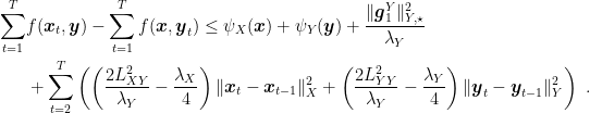
Analogously, we can obtain a version of FTRL that uses the knowledge of the current loss: Be-The-Regularized-Leader (BTRL), that predicts in each time step with ${{\boldsymbol x}_t \in \mathop{\mathrm{argmin}}_{{\boldsymbol x} \in V} \ \psi_t({\boldsymbol x})+\sum_{i=1}^t \ell_i({\boldsymbol x})}$ . In the case that ${\psi_t\equiv 0}$ , then Be-The-Regularized-Leader becomes the Be-The-Leader algorithm. BTRL can be thought as Optimistic FTRL where ${\tilde{\ell}_t=\ell_t}$ . Hence, from the regret of Optimistic FTRL, we immediately have the following theorem.

Theorem 4. Let ${V\subseteq {\mathbb R}^d}$ be convex, closed, and non-empty. Assume for ${t=1, \dots, T}$ that ${\psi_{t} + \sum_{i=1}^{t} \ell_i}$ is proper, closed, and ${\lambda_t}$ -strongly convex w.r.t. ${\|\cdot\|}$ . Then, for all ${{\boldsymbol u} \in V}$ we have

$\displaystyle \sum_{t=1}^T \ell({\boldsymbol x}_t) + \sum_{t=1}^T \ell_t({\boldsymbol u})\\ \leq \psi_{T+1}({\boldsymbol u}) - \psi_{1}({\boldsymbol x}_1) - \sum_{t=1}^T \left(-\frac{\lambda_t}{2} \|{\boldsymbol x}_t-{\boldsymbol x}_{t+1}\|^2 +\psi_t({\boldsymbol x}_{t+1}) - \psi_{t+1}({\boldsymbol x}_{t+1})\right) ~.$

Remark 2. In the Be-The-Leader algorithm, if all the ${\lambda_t=0}$ , then the theorem states that the regret is non-positive.

Notably, the non-negative gradients terms are missing in the bound of BTRL, but we still have the negative ones associated to the change in ${{\boldsymbol x}_t}$ .

Using, for example, BTRL for the ${X}$ -player and Optimistic FTRL for the ${Y}$ -player, we have

$\displaystyle \begin{aligned} \sum_{t=1}^T &f({\boldsymbol x}_t,{\boldsymbol y}) - \sum_{t=1}^T f({\boldsymbol x},{\boldsymbol y}_t) \leq \psi_X({\boldsymbol x}) + \psi_Y({\boldsymbol y}) +\frac{\|{\boldsymbol g}^Y_1\|^2_{Y,\star}}{\lambda_Y}\\ &+ \sum_{t=2}^T \left(\left(\frac{2L^2_{XY}}{\lambda_Y}-\frac{\lambda_X}{4}\right) \|{\boldsymbol x}_t-{\boldsymbol x}_{t-1}\|^2_X + \left(\frac{2L^2_{YY}}{\lambda_Y}-\frac{\lambda_Y}{4}\right) \|{\boldsymbol y}_t-{\boldsymbol y}_{t-1}\|^2_Y\right)~. \end{aligned}$

3. Code and Experiments

This time I will also show some empirical experiments. In fact, I decided to write a small online learning library in Python, to quickly test old and new algorithms. It is called PyOL (Python Online Learning) and you can find it on GitHub and on PyPI, and install it with pip. I designed it in a modular way: you can use FTRL or OMD and choose the projection you want, the learning rates, the hints, etc. I implemented some online learning algorithms, projections, learning rate, reductions, but I plan to add more. At the moment there is no documentation, but I plan to add it and probably I’ll also blog about it.

The Python notebook below will show the effect of optimism in Exponentiated Gradient when used to solve a 2×2 bilinear saddle-point problem with simplex contraints. You can see as the optimistic algorithm converges faster, with both and averaged last solutions. Moreover, even if we did not prove it, the last iterate of the optimistic algorithm converges to the saddle point, while the one of the non-optimistic algorithm goes farther and farther away from the saddle-point.

Sorry, something went wrong. Reload?

Sorry, we cannot display this file.

Sorry, this file is invalid so it cannot be displayed.

view raw bilinear_test.ipynb hosted with ❤ by GitHub

That’s all for this time!
We won’t see other saddle-point results for a while, time to cover new topics.

4. History Bits

Daskalakis et al. (2011) proposed the first no-regret algorithm that achieved a rate of ${O(\frac{\ln T}{T})}$ for the duality gap when used by the two players of a zero-sum game without any communication between the players. However, the algorithm was rather complex and they posed the problem of obtaining the same or faster rate with a simpler algorithm. Rakhlin and Sridharan (2013) solved this problem showing that two Optimistic OMD algorithms can solve the problem in a simpler way, proving a version of Theorems 1 and 2. The possibility to achieve constant regret for each player observed after Theorem 1 is from Luo (2022).

The use of Prescient Online Mirror Descent in saddle-point optimization is from Wang et al. (2021), but renaming ${{\boldsymbol x}_{t}}$ to ${{\boldsymbol x}_{t+1}}$ it is also equivalent to implicit online mirror descent (Kivinen and Warmuth, 1997)(Kulis Bartlett, 2010). In fact, Theorem 3 is from the guarantee of implicit online mirror descent in Campolongo and Orabona (2020).

There is also a tight connection between optimistic updates using the previous gradients and classic approaches to solve saddle-point optimization. In fact, Gidel et al. (2019) showed that using two optimistic gradient descent algorithms to solve a saddle-point problem can be seen as a variant of the Extra-gradient updates (Korpelevich, G. M., 1976), while Mokhtari et al. (2020) show that they can be interpreted as an approximated proximal point algorithm.

Regarding the convergence of the iterations of optimistic algorithms, Daskalakis et al. (2018) proved the convergence of the last iterate to a neighboorhood of the saddle-point in the unconstrained case when using two optimistic online gradient descent algorithms with fixed and small enough stepsizes. Liang and Stokes (2019) improved their result showing that if in addition the matrix ${A}$ is square and full-rank then the iterates of two optimistic online gradient descent will converge exponentially fast to the saddle-point ${(\boldsymbol{0},\boldsymbol{0})}$ . Later, Daskalakis and Panageas (2019) proved the asympototic convergence of optimisitc OMD/FTRL EG with fixed stepsize for the bilinear games over the probability simplex, assuming a unique saddle-point. Wei et al. (2021) proved an exponential rate for the same algorithm under the same assumptions. Finally, Lee et al. (2021, Theorem 4) proved that the iterates of Optimistic OMD with a constant and small enough learning rate asymptotic converge to a saddle-point, without assuming a unique saddle-point.

Acknowledgements

Thanks to Haipeng Luo and Aryan Mokhtari for comments and references.

2 Comments

Fabian says:

November 17, 2022 at 7:58 AM

thanks for this series, they are super useful !

LikeLiked by 1 person

1. bremen79 says:
  
  November 17, 2022 at 5:29 PM
  
  Thank you Fabian! Your blog is also fantastic!
  
  LikeLike

Parameter-free Learning and Optimization Algorithms

Saddle-Point Optimization With Optimism

2 Comments

Leave a Reply Cancel reply

Share this:

Like this:

Related

Leave a Reply Cancel reply