Last Iterate of SGD Converges (Even in Unbounded Domains)

In this blog (and in our ICML 2020 tutorial) we have often discussed the issue of how to tune learning rates in Stochastic (sub)Gradient Descent (SGD). This issue is delicate and sometimes a student might not realize its complexity due to the use of the simplifying assumption of bounded domains.

darkside

Don’t get me wrong: assuming bounded domains is perfectly fine and justified most of the time. However, sometimes it is unnecessary and it might also obscure critical issues in the analysis, as in this case. So, to balance the universe of first-order methods, I decided to show how to easily prove the convergence of the iterates in SGD, even in unbounded domains.

Technically speaking, the following result might be new, but definitely not worth a fight with Reviewer 2 to publish it somewhere.

1. Setting

First, let’s define our setting. We want to solve the following optimization problem

$\displaystyle \min_{{\boldsymbol x} \in V} \ F({\boldsymbol x}),$

where ${V\subseteq {\mathbb R}^d}$ and ${F}$ is a convex function. Now, various assumptions are possible on ${F}$ and choosing the right one depends on your particular problem, there are not right answers. Here, we will not make any strong assumption on ${F}$ . Also, we will not assume ${V}$ to be bounded. Indeed, in most of the modern applications in Machine Learning, ${V}$ is simply the entire space ${{\mathbb R}^d}$ . We will also assume that ${\mathop{\mathrm{argmin}}_{{\boldsymbol x} \in V} \ F({\boldsymbol x})}$ is not empty and ${{\boldsymbol x}^\star}$ is any element in it.

We also assume to have access to a first-order stochastic oracle that returns stochastic sub-gradients of ${F}$ on any point ${{\boldsymbol x}}$ . In formulas, we get ${{\boldsymbol g}({\boldsymbol x},\xi)}$ such that ${\mathop{\mathbb E}_\xi[{\boldsymbol g}({\boldsymbol x},\xi)] \in \partial F({\boldsymbol x})}$ . Practically speaking, every time you calculate the (sub)gradient on a minibatch of training data, that is a stochastic (sub)gradient and roughly speaking the random minibatch is the random variable ${\xi}$ .

Here, for didactic reasons, we will assume that ${{\mathop{\mathbb E}}_\xi[\|{\boldsymbol g}({\boldsymbol x},\xi)\|^2_2]}$ is bounded by 1; similar results can be also show with more realistic assumptions. This holds, for example, if ${F}$ is an average of 1-Lipschitz functions and you draw some of them to calculate the stochastic subgradient.

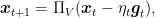
The algorithm we want to focus on is SGD. So, what is SGD? SGD is an incredibly simple optimization algorithm, almost primitive. Indeed, part of its fame depends critically on its simplicity. Basically, you start from a certain ${{\boldsymbol x}_1}$ and you update your solution iteratively moving in the direction of the negative stochastic subgradients, multiplied by a learning rate ${\eta_t}$ . We also use a projection onto ${V}$ . Of course, if ${V={\mathbb R}^d}$ no projection is needed. So, the update of SGD is

$\displaystyle {\boldsymbol x}_{t+1}=\Pi_V({\boldsymbol x}_t -\eta_t {\boldsymbol g}_t),$

where ${{\boldsymbol g}_t:={\boldsymbol g}({\boldsymbol x}_t, \xi_t)}$ and ${\Pi_V}$ is the projection onto ${V}$ . Remember that when you use subgradients, SGD is not a descent algorithm: I already blogged about the fact that the common intuition of moving towards a descent direction is wrong when you use subgradients.

2. Convergence of the Average of the Iterates

Now, the most common analysis of SGD can be done in two different ways: constant learning rate and non-increasing learning rate. We already saw both of them in my lecture notes on online learning, so let’s summarize here the one-step inequality for SGD we need:

$\displaystyle \label{eq:one_step} \eta_t {\mathop{\mathbb E}}[F({\boldsymbol x}_t) - F({\boldsymbol u})] \leq \frac{1}{2}{\mathop{\mathbb E}}[\|{\boldsymbol u}-{\boldsymbol x}_t\|^2] - \frac{1}{2}{\mathop{\mathbb E}}[\|{\boldsymbol u}-{\boldsymbol x}_{t+1}\|^2] + \eta^2_t {\mathop{\mathbb E}}[\|{\boldsymbol g}_t\|^2], \ \ \ \ \ (1)$

for all ${{\boldsymbol u} \in V}$ measureable w.r.t. ${{\boldsymbol x}_1, \dots, {\boldsymbol x}_{t-1}}$ .
If you plan to use ${T}$ iterations, you can you use a learning rate ${\eta = \frac{\alpha}{\sqrt{T}}}$ , and summing (1) we get

$\displaystyle \sum_{t=1}^T \left(\mathop{\mathbb E}[F({\boldsymbol x}_t)] - F({\boldsymbol x}^\star)\right) \leq \frac{\sqrt{T}}{2}\left(\frac{\|{\boldsymbol x}^\star-{\boldsymbol x}_1\|^2}{\alpha} + \alpha\right),$

where we set ${{\boldsymbol u}={\boldsymbol x}^\star}$ . This is not a convergence results yet, because it just says that on average we are converging. To extract a single solution, we can use Jensen’s inequality and obtain

$\displaystyle \mathop{\mathbb E}[F(\bar{{\boldsymbol x}}_T)] \leq F({\boldsymbol x}^\star) + \frac{1}{2\sqrt{T}}\left(\frac{\|{\boldsymbol x}^\star-{\boldsymbol x}_1\|^2}{\alpha} + \alpha\right),$

where ${\bar{{\boldsymbol x}}_T=\frac1T \sum_{t=1}^T {\boldsymbol x}_t}$ . In words, we show a convergence guarantee for the average of the iterates of SGD, not for the last one.

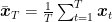
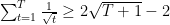
Constant learning rates are a bit annoying because they depends on how many iterations you plan to do, theoretically and empirically. So, let’s now take a look at non-increasing learning rates, ${\eta_t=\frac{\alpha}{\sqrt{t}}}$ . In this case, the correct way to analyze SGD without the bounded assumption is to sum (1) without dividing by ${\eta_t}$ , to have

$\displaystyle \begin{aligned} \sum_{t=1}^T \eta_t \left(\mathop{\mathbb E}[F({\boldsymbol x}_t)] - F({\boldsymbol x}^\star) \right) &\leq \frac{\|{\boldsymbol x}^\star-{\boldsymbol x}_1\|^2}{2} + \frac{1}{2} \sum_{t=1}^T \eta_t^2 \\ &\leq \frac{\|{\boldsymbol x}^\star-{\boldsymbol x}_1\|^2}{2} + \frac{\alpha^2}{2} (\ln T+1), & (2) \\\end{aligned}$

where we set ${{\boldsymbol u}={\boldsymbol x}^\star}$ . From this one, we have two alternatives. First, we can observe that

$\displaystyle \sum_{t=1}^T \eta_t \left(\mathop{\mathbb E}[F({\boldsymbol x}_t)] - F({\boldsymbol x}^\star) \right) \geq \eta_T \sum_{t=1}^T \left(\mathop{\mathbb E}[F({\boldsymbol x}_t)] - F({\boldsymbol x}^\star) \right),$

because ${{\boldsymbol x}^\star}$ is a minimizer and the learning rate non-increasing. So, using again Jensen’s inequality, we get

$\displaystyle \mathop{\mathbb E}[F(\bar{{\boldsymbol x}}_T)] \leq F({\boldsymbol x}^\star) + \frac{\|{\boldsymbol x}^\star-{\boldsymbol x}_1\|^2}{2 \alpha \sqrt{T}} + \frac{\alpha (\ln T+1)}{2\sqrt{T}}~.$

Note that if you like these sorts of games, you can even change the learning rate to shave a ${\sqrt{\ln T}}$ factor, but it is probably useless from an applied point of view.

Another possibility is to use a weighted average:

$\displaystyle \begin{aligned} \mathop{\mathbb E}[F(\bar{{\boldsymbol x}}'_T)] &\leq F({\boldsymbol x}^\star) + \frac{\|{\boldsymbol x}^\star-{\boldsymbol x}_1\|^2 + \alpha^2 (\ln T+1)}{2 \sum_{t=1}^T \eta_t} \\ &\leq F({\boldsymbol x}^\star) + \frac{1}{4\sqrt{T+1}-4}\left(\frac{\|{\boldsymbol x}^\star-{\boldsymbol x}_1\|^2}{\alpha} + \alpha (\ln T+1)\right), \end{aligned}$

where ${\bar{{\boldsymbol x}}'_T=\frac{1}{\sum_{t=1}^T \eta_t} \sum_{t=1}^T \eta_t {\boldsymbol x}_t}$ and we used ${\sum_{t=1}^T \frac{1}{\sqrt{t}}\geq 2 \sqrt{T+1}-2}$ . Note that this option does not seem to give any advantage over the unweighted average above. Also, it weights the first iterations more than the last ones, that in most of the cases is a bad idea: First iterations tend to be farther away from the optimum then the last ones.

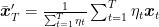
Let’s summarize what we have till now:

Unbounded domains are fine with both constant and time-varying learning rates.
The optimal learning rate depends on the distance between the optimal solution and the initial iterate, because the optimal setting of ${\alpha}$ is proportional to ${\|{\boldsymbol x}_1-{\boldsymbol x}^\star\|_2}$ .
The weighted average is probably a bad idea and not strictly necessary.
It seems we can only guarantee convergence for (weighted) averages of iterates.

The last point is a bit concerning: most of the time we take the last iterate of SGD, why we do it if the theory applies to the average?

3. Convergence of the Last Iterate

Actually, we do know that

the last solution of SGD converges in unbounded domains with constant learning rate (Zhang, T., 2004).
the last iterate of SGD converges in bounded domains with non-increasing learning rates (Shamir, O. and Zhang, T., 2013).

So, what about unbounded domains and non-increasing learning rate, i.e., 90% of the uses of SGD? It turns out that it is equally simple and I think the proof is also instructive! As surprising as it might sound, not dividing by ${\eta_t}$ (1) is the key ingredient we need. The proof plan is the following: we want to prove that the value of ${F}$ on the last iterate ${{\boldsymbol x}_T}$ is not too far from the value of ${F}$ on ${\bar{{\boldsymbol x}}_T}$ . To prove it, we need the following technical lemma on sequences of non-negative numbers multiplied by non-increasing learning rates, whose proof is in the Appendix. This Lemma relates the last element of a sequence of numbers to their average.

Lemma 1. Let ${\eta_t, \ t=1,\cdots, T}$ a non-increasing sequence of positive numbers and ${q_t \geq0, t=1, \cdots,T}$ . Then

$\displaystyle \eta_T q_T \leq \frac{1}{T} \sum_{t=1}^T \eta_t q_t + \sum_{k=1}^{T-1} \frac{1}{k(k+1)} \sum_{t=T-k+1}^T \eta_t (q_t - q_{T-k})~.$

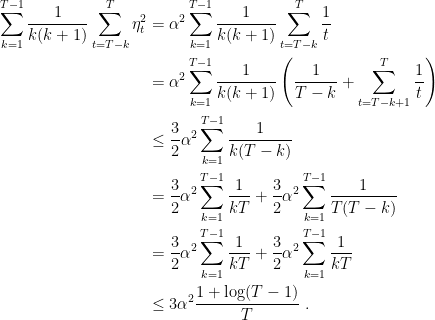
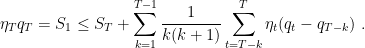
With the above Lemma, we can prove the following guarantee for the convergence of the last iterate of SGD.

Theorem 2. Assume the stepsizes deterministic and non-increasing. Then

$\displaystyle \label{eq:thm_last_one} \eta_T \left(\mathop{\mathbb E}[F({\boldsymbol x}_T)]-F({\boldsymbol x}^\star)\right) \leq \frac{1}{T} \sum_{t=1}^T \eta_t \left(\mathop{\mathbb E}[F({\boldsymbol x}_t)]-F({\boldsymbol x}^\star)\right) + \frac{1}{2} \sum_{k=1}^{T-1} \frac{1}{k (k+1)}\sum_{t=T-k}^T \eta^2_t\mathop{\mathbb E}[\|{\boldsymbol g}_t\|^2_2]~. \ \ \ \ \ (3)$

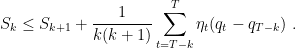
Proof: We use Lemma 1, with ${q_t=\mathop{\mathbb E}[F({\boldsymbol x}_t)]-F({\boldsymbol x}^\star)}$ , to have

$\displaystyle \begin{aligned} \eta_T \left(\mathop{\mathbb E}[F({\boldsymbol x}_t)]-F({\boldsymbol x}^\star)\right) \leq \frac{1}{T} \sum_{t=1}^T \eta_t \mathop{\mathbb E}[F({\boldsymbol x}_t)-F({\boldsymbol x}^\star)] + \sum_{k=1}^{T-1} \frac{1}{k(k+1)} \sum_{t=T-k+1}^T \eta_t \mathop{\mathbb E}[F({\boldsymbol x}_t) - F({\boldsymbol x}_{T-k})]~. \end{aligned}$

Now, we bound the sum in the r.h.s. of last inequality. Summing (1) from ${T-k}$ to ${T}$ , we have the following inequality that holds for any ${{\boldsymbol u} \in V}$ :

$\displaystyle \begin{aligned} \sum_{t=T-k}^T \eta_t \mathop{\mathbb E}[F({\boldsymbol x}_t)-F({\boldsymbol u})] \leq \frac12 \mathop{\mathbb E}[\|{\boldsymbol x}_{T-k}-{\boldsymbol u}\|^2] + \frac{1}{2}\sum_{t=T-k}^T \eta^2_t \mathop{\mathbb E}[\|{\boldsymbol g}_t\|^2_2]~. \end{aligned}$

Hence, setting ${{\boldsymbol u}={\boldsymbol x}_{T-k}}$ , we have

$\displaystyle \sum_{t=T-k+1}^T \eta_t \mathop{\mathbb E}[F({\boldsymbol x}_t)-F({\boldsymbol x}_{T-k})] =\sum_{t=T-k}^T \eta_t \mathop{\mathbb E}[F({\boldsymbol x}_t)-F({\boldsymbol x}_{T-k})] \leq \frac{1}{2}\sum_{t=T-k}^T \eta^2_t \mathop{\mathbb E}[\|{\boldsymbol g}_t\|^2_2]~.$

Putting all together, we have the stated bound. $\Box$

There are a couple of nice tricks in the proof that might be interesting to study carefully. First, we use the fact that one-step inequality in (1) holds for any ${{\boldsymbol u} \in V}$ . Most of the time, we state it with ${{\boldsymbol u}}$ equal to ${{\boldsymbol x}^\star}$ , but it turns out that the more general statement is actually important! In fact, it is possible to know how far is the performance of last iterate from the performance of the average because the incremental nature of SGD makes possible to know exactly how far is ${{\boldsymbol x}_t}$ from any previous iterate ${{\boldsymbol x}_i}$ , with ${i<t}$ . Please note that all of this would be hidden in the case of bounded domains, where all the distances are bounded by the diameter of the set, and you don’t get the dependency on ${\|{\boldsymbol x}_t-{\boldsymbol u}\|_2^2}$ .

Now we have all the ingredients and we only have to substitute a particular choice of the learning rate.

Corollary 3. Assume ${T\geq2}$ , ${{\mathop{\mathbb E}}_t[\|{\boldsymbol g}_t\|^2_2]\leq 1}$ and ${\eta_t=\frac{\alpha}{\sqrt{t}}}$ for ${t=1, \dots, T}$ . Then, we have

$\displaystyle \mathop{\mathbb E}[F({\boldsymbol x}_T)]-F({\boldsymbol x}^\star) \leq \frac{1}{2\sqrt{T}} \left(\frac{\|{\boldsymbol x}^\star-{\boldsymbol x}_1\|^2}{\alpha} + \alpha (\ln T+1)\right) + \frac{3\alpha}{2} \frac{1+\log(T-1)}{\sqrt{T}}~.$

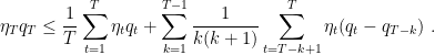
Proof: First, observe that

$\displaystyle \sum_{t=T-k+1}^T \frac1t \leq \int_{T-k}^T \frac{1}{t}dt=\log\frac{T}{T-k} = \log \left(1+\frac{k}{T-k}\right) \leq \frac{k}{T-k}~.$

Now, considering the last term in (3), we have

$\displaystyle \begin{aligned} \sum_{k=1}^{T-1} \frac{1}{k (k+1)}\sum_{t=T-k}^T \eta^2_t &= \alpha^2 \sum_{k=1}^{T-1} \frac{1}{k (k+1)} \sum_{t=T-k}^{T} \frac1t \\ &= \alpha^2 \sum_{k=1}^{T-1} \frac{1}{k (k+1)} \left(\frac{1}{T-k} + \sum_{t=T-k+1}^{T} \frac1t \right) \\ &\leq \frac{3}{2}\alpha^2 \sum_{k=1}^{T-1} \frac{1}{k (T-k)} \\ &= \frac{3}{2}\alpha^2 \sum_{k=1}^{T-1} \frac{1}{k T} + \frac{3}{2}\alpha^2\sum_{k=1}^{T-1} \frac{1}{T(T-k)} \\ &= \frac{3}{2}\alpha^2 \sum_{k=1}^{T-1} \frac{1}{k T} + \frac{3}{2}\alpha^2\sum_{k=1}^{T-1} \frac{1}{k T} \\ &\leq 3\alpha^2 \frac{1+\log(T-1)}{T}~. \end{aligned}$

Using (2) and dividing by ${\eta_T}$ , we have the stated bound. $\Box$

Note that the above proof works similarly if ${\eta_t=\eta=\frac{\alpha}{\sqrt{T}}}$ .

4. History Bits

The first finite-time convergence proof for the last iterate of SGD is from (Zhang, T., 2004), where he considered the constant learning rate case. It was later extended in (Shamir, O. and Zhang, T., 2013) for time-varying learning rates but only for bounded domains. The convergence rate for the weighted average in unbounded domains is from (Zhang, T., 2004). The observation that the weighted average is not needed and the plain average works equally well for non-increasing learning rates is from (X. Li and F. Orabona, 2019), where we needed it for the particular case of AdaGrad learning rates. The idea of analyzing SGD without dividing by the learning rate is by (Zhang, T., 2004). Lemma 1 is new but actually hidden in the the convergence proof of the last iterate of SGD with linear predictors and square losses in (Lin, J. and Rosasco, L. and Zhou, D.-X., 2016), that in turn is based on the one in (Shamir, O. and Zhang, T., 2013). As far as I know, Corollary 3 is new, but please let me know if you happen to know a reference for it! It is possible to remove the logarithmic term in the bound using a different learning rate, but the proof is only for bounded domains (Jain, P. and Nagaraj, D. and Netrapalli, P., 2019).

5. Exercises

Exercise 1. Generalize the above proofs to the Stochastic Mirror Descent case.

Exercise 2. Remove the assumption of expected bounded stochastic subgradients and instead assume that ${F}$ is ${L}$ -smooth, i.e., has ${L}$ -Lipschitz gradient, and the variance of the noise is bounded. Hint: take a look at the proofs in (Zhang, T., 2004) and (X. Li and F. Orabona, 2019)

6. Appendix

Proof of Lemma 1: Define ${S_k:=\frac1k \sum_{t=T-k+1}^T \eta_t q_t}$ , so we have

$\displaystyle \sum_{t=T-k}^T \eta_t (q_t - q_{T-k}) \geq \sum_{t=T-k}^T (\eta_t q_t - \eta_{T-k} q_{T-k}) = (k+1) S_{k+1} - \eta_{T-k} (k+1) q_{T-k},$

that implies

$\displaystyle S_{k+1} - \eta_{T-k} q_{T-k} \leq \frac{1}{k+1} \sum_{t=T-k}^T \eta_t (q_t - q_{T-k})~.$

Now, from the definition of ${S_k}$ and the above inequality, we have

$\displaystyle k S_k = (k+1) S_{k+1} - \eta_{T-k} q_{T-k} = k S_{k+1} + S_{k+1} - \eta_{T-k} q_{T-k} \leq k S_{k+1} + \frac{1}{k+1} \sum_{t=T-k}^T \eta_t (q_t - q_{T-k}),$

that implies

$\displaystyle S_{k} \leq S_{k+1} + \frac{1}{k(k+1)} \sum_{t=T-k}^T \eta_t (q_t - q_{T-k})~.$

Unrolling the inequality, we have

$\displaystyle \eta_T q_T = S_1 \leq S_T + \sum_{k=1}^{T-1} \frac{1}{k(k+1)} \sum_{t=T-k}^T \eta_t (q_t - q_{T-k})~.$

Using the definition of ${S_T}$ and the fact that ${\sum_{t=T-k}^T \eta_t (q_t - q_{T-k})=\sum_{t=T-k+1}^T \eta_t (q_t - q_{T-k})}$ , we have the stated bound. $\Box$

4 Comments

bremen79 says:

August 8, 2020 at 8:33 AM

EDIT: inspired by the discussion on Twitter, I added exercise 2.

LikeLike

Ali Siahkamari says:

April 23, 2021 at 11:21 PM

Very interesting! My first guess for why the last iterate should converge was that $x_T$ is close to $\bar x_T$. However for a simple one dimensional case where all $g_t = 1$, it can be shown that $x_T- \bar x_T = O(\sqrt(T))$.

LikeLike

1. bremen79 says:
  
  April 26, 2021 at 3:18 PM
  
  Interesting! Can you sketch your construction?
  
  LikeLike
  
  1. Ali Siahkamari says:
    
    April 30, 2021 at 12:00 AM
    
    I was thinking $x_T = -\sum_{t=1}^{T-1} \alpha g_t/\sqrt{t}$. Then we get $\bar x_T =-1/T\sum_{k=1}^T\sum_{t=1}^{k-1} \alpha g_t/\sqrt{t}$. Now by assuming $g_t=1$ and simplifying $x_t- \bar x_T$ it is easy to show that it is of the order $O(\sqrt{T})$. Though the problem is the loss functions seems unbounded and $\bar x_t$ actually doesn’t converge! So I was totally wrong.
    
    LikeLiked by 1 person
Pingback: A Simple Proof for Optimistic OMD – Parameter-free Learning and Optimization Algorithms

Share this:

Related

Leave a comment Cancel reply