In this post, we will see some connections between saddle-point problems and Game Theory, as well as with Boosting.
Warning: this post heavily needs the knowledge of the min-max problems. So, I strongly suggest to read the previous one before, if you do not remember it.
1. Game-Theory interpretation of Saddle-Point Problems
An instantiation of a saddle-point problems also has an interpretation in Game Theory as a Two-player Zero-Sum Game. Note that Game Theory is a vast field and two-person zero-sum games are only a very small subset of the problems in this domain and what I describe here is an even smaller subset of this subset of problems.
Game theory studies what happens when self-interested agents interact. By self-interested, we mean that each agent has an ideal state of things he wants to reach, that can include a description of what should happen to other agents as well, and he works towards this goal. In two-person games the players act simultaneously and then they receive their losses. In particular, the 


We consider the so-called two-person normal-form games, that is when the first player has 


A fundamental concept in game theory is the one of Nash Equilibrium. We have a Nash equilibrium if all players are playing their best strategy to the other players’ strategies. That is, none of the players has incentive to change their strategy if the other player does not change it. For the zero-sum two-person game, this can be formalized saying that 

This is exactly the definition of saddle-point for the function 

For zero-sum two-person game the Nash equilibrium has an immediate interpretation: From the definiton above, if the first player uses the strategy 


Example 1 (Cake cutting). Suppose to have a game between two people: The first player cuts the cake in two and the second one chooses a piece; the first player receives the piece that was not chosen. We can formalize it with the following matrix
larger piece smaller piece cut evenly 0 0 cut unevenly 10 -10 When the first player plays action
, the first player receives the loss
and the second player receives
. The losses represent how much less in percentage compared to half of the cake the first player is receiving. The second player receives the negative of the same number. It should be easy to convince oneself that the strategy pair is
is an equilibrium with value of the game of 0.
Example 2 (Rock-paper-scissors). Let’s consider the game of Rock-paper-scissors. We describe it with the following matrix
Rock Paper Scissors Rock 0 1 -1 Paper -1 0 1 Scissors 1 -1 0 It should be immediate to realize that there are no pure Nash equilibria for this game. However, there is a mixed Nash equilibrium when each player randomize the action with a uniform probability distribution and value of the game equal to 0.
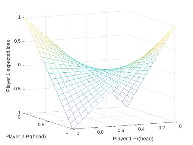
Example 3 (Matching Pennies). In this game, both players show a face of a penny. If the two faces are the same, the first player wins both, otherwise the second player wins both. The associated matrix
head tail head -1 1 tail 1 -1 It is easy to see that the Nash equilibrium is when both players randomize the face to show with equal probability.
In this simple case, we can visualize the saddle point associated to this problem in Figure 1
Unless the game is very small, we find Nash equilibria using numerical procedures that typically give us only approximate solutions. Hence, as for 

Obviously, any Nash equilibrium is also an
From what we said last time, it should be immediate to see how to numerically calculate the Nash equilibrium of a two-person zero-sum game. In fact, we know that we can use online convex optimization algorithms to find 

2. Boosting as a Two-Person Game
We will now show that the Boosting problem can also be seen as the solution of a zero-sum two-person game. In fact, this is my favorite explanation of Boosting because it focuses on the problem rather than on a specific algorithm.
Let 


The aim of boosting is to find a combination of the functions in 


First, we construct a matrix of the misclassifications for each function: 


Given the definition of the matrix
![\displaystyle \min_{{\boldsymbol p} \in \Delta^n} \max_{{\boldsymbol q} \in \Delta^m} \ \sum_{i=1}^n \sum_{i=1}^m p_i q_j \boldsymbol{1}[h_i({\boldsymbol z}_j)\neq y_j]~.](https://s0.wp.com/latex.php?latex=%5Cdisplaystyle+%5Cmin_%7B%7B%5Cboldsymbol+p%7D+%5Cin+%5CDelta%5En%7D+%5Cmax_%7B%7B%5Cboldsymbol+q%7D+%5Cin+%5CDelta%5Em%7D+%5C+%5Csum_%7Bi%3D1%7D%5En+%5Csum_%7Bi%3D1%7D%5Em+p_i+q_j+%5Cboldsymbol%7B1%7D%5Bh_i%28%7B%5Cboldsymbol+z%7D_j%29%5Cneq+y_j%5D%7E.+&bg=ffffff&fg=000000&s=0&c=20201002)
Let’s now formalize the assumption on the functions: We assume the existence of a weak learning oracle that for any 

![\displaystyle {\boldsymbol e}_{i^\star}^\top M {\boldsymbol q} = \sum_{j=1}^m q_j \boldsymbol{1}[h_{i^\star}({\boldsymbol z}_j)\neq y_j] \leq \frac{1}{2} - \gamma,](https://s0.wp.com/latex.php?latex=%5Cdisplaystyle+%7B%5Cboldsymbol+e%7D_%7Bi%5E%5Cstar%7D%5E%5Ctop+M+%7B%5Cboldsymbol+q%7D+%3D+%5Csum_%7Bj%3D1%7D%5Em+q_j+%5Cboldsymbol%7B1%7D%5Bh_%7Bi%5E%5Cstar%7D%28%7B%5Cboldsymbol+z%7D_j%29%5Cneq+y_j%5D+%5Cleq+%5Cfrac%7B1%7D%7B2%7D+-+%5Cgamma%2C+&bg=ffffff&fg=000000&s=0&c=20201002)
where 
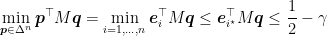
and

we have that the value of the game satisfies 


![\displaystyle \label{eq:boosting_eq1} \sum_{i=1}^n p^\star_i \boldsymbol{1}[h_i({\boldsymbol z}_j) \neq y_j] = ({\boldsymbol p}^\star)^\top M {\boldsymbol e}_j \leq v^\star \leq \frac12 - \gamma < \frac12~. \ \ \ \ \ (1)](https://s0.wp.com/latex.php?latex=%5Cdisplaystyle+%5Clabel%7Beq%3Aboosting_eq1%7D+%5Csum_%7Bi%3D1%7D%5En+p%5E%5Cstar_i+%5Cboldsymbol%7B1%7D%5Bh_i%28%7B%5Cboldsymbol+z%7D_j%29+%5Cneq+y_j%5D+%3D+%28%7B%5Cboldsymbol+p%7D%5E%5Cstar%29%5E%5Ctop+M+%7B%5Cboldsymbol+e%7D_j+%5Cleq+v%5E%5Cstar+%5Cleq+%5Cfrac12+-+%5Cgamma+%3C+%5Cfrac12%7E.+%5C+%5C+%5C+%5C+%5C+%281%29&bg=ffffff&fg=000000&s=0&c=20201002)
In words, this means that every sample 


Given what we have said till now, a natural strategy is to use online convex optimization algorithms. In particular, we can use Algorithm 3 from my previous post, where in each round the 
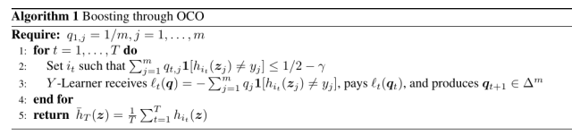
Let’s show a guarantee on the misclassification error of this algorithm. From the second equality of Theorem 6 in my previous post, for any

From the assumption on the weak-learnability oracle, we have 

![{\frac{1}{T} \sum_{t=1}^T {\boldsymbol e}_{i_t}^\top M {\boldsymbol q} = \frac1T \sum_{i=1}^T \boldsymbol{1}[h_{i_t}({\boldsymbol z}_j) \neq y_j]}](https://s0.wp.com/latex.php?latex=%7B%5Cfrac%7B1%7D%7BT%7D+%5Csum_%7Bt%3D1%7D%5ET+%7B%5Cboldsymbol+e%7D_%7Bi_t%7D%5E%5Ctop+M+%7B%5Cboldsymbol+q%7D+%3D+%5Cfrac1T+%5Csum_%7Bi%3D1%7D%5ET+%5Cboldsymbol%7B1%7D%5Bh_%7Bi_t%7D%28%7B%5Cboldsymbol+z%7D_j%29+%5Cneq+y_j%5D%7D&bg=ffffff&fg=000000&s=0&c=20201002)
![\displaystyle \frac1T \sum_{i=1}^T \boldsymbol{1}[h_{i_t}({\boldsymbol z}_j) \neq y_j] \leq \frac12 - \gamma + \frac{\text{Regret}^Y_T({\boldsymbol e}_j)}{T}~.](https://s0.wp.com/latex.php?latex=%5Cdisplaystyle+%5Cfrac1T+%5Csum_%7Bi%3D1%7D%5ET+%5Cboldsymbol%7B1%7D%5Bh_%7Bi_t%7D%28%7B%5Cboldsymbol+z%7D_j%29+%5Cneq+y_j%5D+%5Cleq+%5Cfrac12+-+%5Cgamma+%2B+%5Cfrac%7B%5Ctext%7BRegret%7D%5EY_T%28%7B%5Cboldsymbol+e%7D_j%29%7D%7BT%7D%7E.+&bg=ffffff&fg=000000&s=0&c=20201002)
If 

In this scheme, we construct 

Let’s now instantiate this framework with a specific OCO algorithm. For example, using Exponentiated Gradient (EG) as algorithm for the 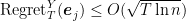

Boosting and Margins What happens if we keep boosting after the training error reaches 0? It turns out we maximize the margin, defined as 
![{\boldsymbol{1}[h_{i_t}({\boldsymbol z}_j)\neq y_j] = \frac{1-y_j h_{i_t}({\boldsymbol z}_j)}{2}}](https://s0.wp.com/latex.php?latex=%7B%5Cboldsymbol%7B1%7D%5Bh_%7Bi_t%7D%28%7B%5Cboldsymbol+z%7D_j%29%5Cneq+y_j%5D+%3D+%5Cfrac%7B1-y_j+h_%7Bi_t%7D%28%7B%5Cboldsymbol+z%7D_j%29%7D%7B2%7D%7D&bg=ffffff&fg=000000&s=0&c=20201002)

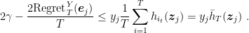
Hence, when the number of rounds goes to infinity the minimum margin on the training samples reaches 
The above reduction does not tell us how the training error precisely behaves. However, we can get this information changing the learning with expert algorithm. Indeed, if you read my old posts you should know that there are learning with experts algorithm provably better than EG. We can use a learning with experts algorithm that guarantees a regret 


Using the expression of the regret, we have that the fraction of misclassification errors 

3. History Bits
The reduction from boosting to two-person game and learning with expert is from Freund and Schapire (1996). It seems that the question if a weak learner can be boosted into a strong learner was originally posed by Kearns and Valiant (1988) (see also Kearns (1988)) but I could not verify this claim because I could not find their technical report anywhere. It was answered in the positive by Schapire (1990). The AdaBoost algorithm is from Freund and Schapire (1997). The idea of using algorithms that guarantee a KL regret bound in (2) is from Luo and Schapire (2014).
Acknowledgements
Thanks to Nicolò Campolongo for hunting down my typos.

Very interesting and comprehensive.
LikeLiked by 1 person