This post is part of the lecture notes of my class “Introduction to Online Learning” at Boston University, Fall 2019.
You can find all the lectures I published here.
Throughout this class, we considered the adversarial model as our model of the environment. This allowed us to design algorithm that work in this setting, as well as in other more benign settings. However, the world is never completely adversarial. So, we might be tempted to model the environment in some way, but that would leave our algorithm vulnerable to attacks. An alternative, is to consider the data as generated by some predictable process plus adversarial noise. In this view, it might be beneficial to try to model the predictable part, without compromising the robustness to the adversarial noise.
In this class, we will explore this possibility through a particular version of Follow-The-Regularized-Leader (FTRL), where we predict the next loss. In very intuitive terms, if our predicted loss is correct, we can expect the regret to decrease. However, if our prediction is wrong we still want to recover the worst case guarantee. Such algorithm is called Optimistic FTRL.
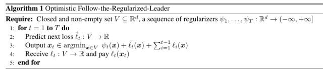
The core idea of Optimistic FTRL is to predict the next loss and use it in the update rule, as summarized in Algorithm 1. Note that for the sake of the analysis, it does not matter how the prediction is generated. It can be even generated by another online learning procedure!
Let’s see why this is a good idea. Remember that FTRL simply predicts with the minimizer of the previous losses plus a time-varying regularizer. Let’s assume for a moment that instead we have the gift of predicting the future, so we do know the next loss ahead of time. Then, we could predict with its minimizer and suffer a negative regret. However, probably our foresight abilities are not so powerful, so our prediction of the next loss might be inaccurate. In this case, a better idea might be just to add our predicted loss to the previous ones and minimize the regularized sum. We would expect the regret guarantee to improve if our prediction of the future loss is precise. At the same time, if the prediction is wrong, we expect its influence to be limited, given that we use it together with all the past losses.
All these intuitions can be formalized in the following Theorem.
Theorem 1 With the notation in Algorithm 1, let
be convex, closed, and non-empty. Denote by
. Assume for
that
is proper and
-strongly convex w.r.t.
,
and
proper and convex, and
. Also, assume that
and
are non-empty. Then, there exists
for
for all
.
![\displaystyle \begin{aligned} \sum_{t=1}^T &\ell({\boldsymbol x}_t) - \sum_{t=1}^T \ell_t({\boldsymbol u})\\ &\leq \psi_{T+1}({\boldsymbol u}) - \psi_{1}({\boldsymbol x}_1) + \sum_{t=1}^T \left[\langle {\boldsymbol g}_t-\tilde{{\boldsymbol g}}_t,{\boldsymbol x}_t-{\boldsymbol x}_{t+1}\rangle -\frac{\lambda_t}{2} \|{\boldsymbol x}_t-{\boldsymbol x}_{t+1}\|^2 +\psi_t({\boldsymbol x}_{t+1}) - \psi_{t+1}({\boldsymbol x}_{t+1})\right] \\ &\leq \psi_{T+1}({\boldsymbol u}) - \psi_{1}({\boldsymbol x}_1) + \sum_{t=1}^T \left[\frac{\| {\boldsymbol g}_t-\tilde{{\boldsymbol g}}_t\|_\star^2}{2\lambda_t} +\psi_t({\boldsymbol x}_{t+1}) - \psi_{t+1}({\boldsymbol x}_{t+1})\right], \end{aligned}](https://s0.wp.com/latex.php?latex=%5Cdisplaystyle+%5Cbegin%7Baligned%7D+%5Csum_%7Bt%3D1%7D%5ET+%26%5Cell%28%7B%5Cboldsymbol+x%7D_t%29+-+%5Csum_%7Bt%3D1%7D%5ET+%5Cell_t%28%7B%5Cboldsymbol+u%7D%29%5C%5C+%26%5Cleq+%5Cpsi_%7BT%2B1%7D%28%7B%5Cboldsymbol+u%7D%29+-+%5Cpsi_%7B1%7D%28%7B%5Cboldsymbol+x%7D_1%29+%2B+%5Csum_%7Bt%3D1%7D%5ET+%5Cleft%5B%5Clangle+%7B%5Cboldsymbol+g%7D_t-%5Ctilde%7B%7B%5Cboldsymbol+g%7D%7D_t%2C%7B%5Cboldsymbol+x%7D_t-%7B%5Cboldsymbol+x%7D_%7Bt%2B1%7D%5Crangle+-%5Cfrac%7B%5Clambda_t%7D%7B2%7D+%5C%7C%7B%5Cboldsymbol+x%7D_t-%7B%5Cboldsymbol+x%7D_%7Bt%2B1%7D%5C%7C%5E2+%2B%5Cpsi_t%28%7B%5Cboldsymbol+x%7D_%7Bt%2B1%7D%29+-+%5Cpsi_%7Bt%2B1%7D%28%7B%5Cboldsymbol+x%7D_%7Bt%2B1%7D%29%5Cright%5D+%5C%5C+%26%5Cleq+%5Cpsi_%7BT%2B1%7D%28%7B%5Cboldsymbol+u%7D%29+-+%5Cpsi_%7B1%7D%28%7B%5Cboldsymbol+x%7D_1%29+%2B+%5Csum_%7Bt%3D1%7D%5ET+%5Cleft%5B%5Cfrac%7B%5C%7C+%7B%5Cboldsymbol+g%7D_t-%5Ctilde%7B%7B%5Cboldsymbol+g%7D%7D_t%5C%7C_%5Cstar%5E2%7D%7B2%5Clambda_t%7D+%2B%5Cpsi_t%28%7B%5Cboldsymbol+x%7D_%7Bt%2B1%7D%29+-+%5Cpsi_%7Bt%2B1%7D%28%7B%5Cboldsymbol+x%7D_%7Bt%2B1%7D%29%5Cright%5D%2C+%5Cend%7Baligned%7D&bg=ffffff&fg=000000&s=0&c=20201002)
Proof: We can interpret the Optimistic-FTRL as FTRL with a regularizer 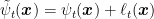

Hence, from the equality for FTRL, we immediately get
![\displaystyle \begin{aligned} \sum_{t=1}^T &\ell({\boldsymbol x}_t) - \sum_{t=1}^T \ell_t({\boldsymbol u}) \\ &\leq \tilde{\ell}_{T+1}({\boldsymbol u}) + \psi_{T+1}({\boldsymbol u}) - \min_{{\boldsymbol x} \in V} \ (\tilde{\ell}_1({\boldsymbol x})+\psi_{1}({\boldsymbol x})) + \sum_{t=1}^T [F_t({\boldsymbol x}_t) - F_{t+1}({\boldsymbol x}_{t+1}) + \ell_t({\boldsymbol x}_t) +\tilde{\ell}_t({\boldsymbol x}_t)-\tilde{\ell}_{t+1}({\boldsymbol x}_{t+1})] \\ &= \psi_{T+1}({\boldsymbol u}) - \psi_{1}({\boldsymbol x}_1) + \sum_{t=1}^T [F_t({\boldsymbol x}_t) - F_{t+1}({\boldsymbol x}_{t+1}) + \ell_t({\boldsymbol x}_t)]~. \end{aligned}](https://s0.wp.com/latex.php?latex=%5Cdisplaystyle+%5Cbegin%7Baligned%7D+%5Csum_%7Bt%3D1%7D%5ET+%26%5Cell%28%7B%5Cboldsymbol+x%7D_t%29+-+%5Csum_%7Bt%3D1%7D%5ET+%5Cell_t%28%7B%5Cboldsymbol+u%7D%29+%5C%5C+%26%5Cleq+%5Ctilde%7B%5Cell%7D_%7BT%2B1%7D%28%7B%5Cboldsymbol+u%7D%29+%2B+%5Cpsi_%7BT%2B1%7D%28%7B%5Cboldsymbol+u%7D%29+-+%5Cmin_%7B%7B%5Cboldsymbol+x%7D+%5Cin+V%7D+%5C+%28%5Ctilde%7B%5Cell%7D_1%28%7B%5Cboldsymbol+x%7D%29%2B%5Cpsi_%7B1%7D%28%7B%5Cboldsymbol+x%7D%29%29+%2B+%5Csum_%7Bt%3D1%7D%5ET+%5BF_t%28%7B%5Cboldsymbol+x%7D_t%29+-+F_%7Bt%2B1%7D%28%7B%5Cboldsymbol+x%7D_%7Bt%2B1%7D%29+%2B+%5Cell_t%28%7B%5Cboldsymbol+x%7D_t%29+%2B%5Ctilde%7B%5Cell%7D_t%28%7B%5Cboldsymbol+x%7D_t%29-%5Ctilde%7B%5Cell%7D_%7Bt%2B1%7D%28%7B%5Cboldsymbol+x%7D_%7Bt%2B1%7D%29%5D+%5C%5C+%26%3D+%5Cpsi_%7BT%2B1%7D%28%7B%5Cboldsymbol+u%7D%29+-+%5Cpsi_%7B1%7D%28%7B%5Cboldsymbol+x%7D_1%29+%2B+%5Csum_%7Bt%3D1%7D%5ET+%5BF_t%28%7B%5Cboldsymbol+x%7D_t%29+-+F_%7Bt%2B1%7D%28%7B%5Cboldsymbol+x%7D_%7Bt%2B1%7D%29+%2B+%5Cell_t%28%7B%5Cboldsymbol+x%7D_t%29%5D%7E.+%5Cend%7Baligned%7D&bg=ffffff&fg=000000&s=0&c=20201002)
Now focus on the terms 


where 


By the definition of dual norms, we also have that


Let’s take a look at the second bound in the theorem. Compared to the similar bound for FTRL, we now have the terms 

Example 1. In the case of linear losses
and strongly convex regularizers, the update of optimistic FTRL becomes
where
and we used the hint
. For example, if
, we have
where
is the projection onto
.


Despite the simplicity of the algorithm and its analysis, there are many applications of this principle. We will only describe a couple of them. Recently, this idea was used even to recover the Nesterov’s acceleration algorithm and to prove faster convergence in repeated games.
1. Regret that Depends on the Variance of the Subgradients
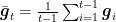
Consider of running Optimistic-FTRL on the linearized losses 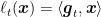


This implies
It is immediate to see that the minimizer is 


Remark 1 Instead of using the mean of the past subgradients, we could use any other strategy or even a mix of different strategies. For example, assuming the subgradients bounded, we could use an algorithm to solve the Learning with Expert problem, where each expert is a strategy. Then, we would obtain a bound that depends on the predictions of the best strategy, plus the regret of the expert algorithm.
2. Online Convex Optimization with Gradual Variations
In this section, we consider the case that the losses we receive have small variations over time. We will show that in this case it is possible to get constant regret in the case that the losses are equal.
In this case, the simple strategy we can use to predict the next subgradient is to use the previous one, that is 


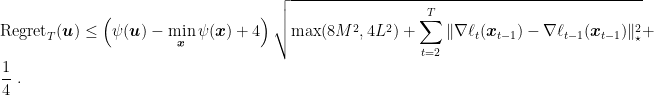
Corollary 2 Under the assumptions of Theorem 1, define
where
is 1-strongly convex w.r.t.
for
, where
is the smoothness constant of the losses
, we have
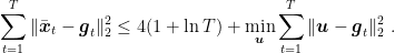
Moreover, assuming
for all
, setting
, we have

Proof: From the Optimistic-FTRL bound with a fixed regularizer, we immediately get
![\displaystyle \sum_{t=1}^T \langle{\boldsymbol g}_t,{\boldsymbol x}_t\rangle - \sum_{t=1}^T \langle {\boldsymbol g}_t, {\boldsymbol u}\rangle \leq \lambda_{T}\psi({\boldsymbol u}) - \lambda_1 \psi({\boldsymbol x}_1) + \sum_{t=1}^T \left[\langle {\boldsymbol g}_t-\tilde{{\boldsymbol g}}_t,{\boldsymbol x}_t-{\boldsymbol x}_{t+1}\rangle -\frac{\lambda_t}{2} \|{\boldsymbol x}_t-{\boldsymbol x}_{t+1}\|^2 \right]~.](https://s0.wp.com/latex.php?latex=%5Cdisplaystyle+%5Csum_%7Bt%3D1%7D%5ET+%5Clangle%7B%5Cboldsymbol+g%7D_t%2C%7B%5Cboldsymbol+x%7D_t%5Crangle+-+%5Csum_%7Bt%3D1%7D%5ET+%5Clangle+%7B%5Cboldsymbol+g%7D_t%2C+%7B%5Cboldsymbol+u%7D%5Crangle+%5Cleq+%5Clambda_%7BT%7D%5Cpsi%28%7B%5Cboldsymbol+u%7D%29+-+%5Clambda_1+%5Cpsi%28%7B%5Cboldsymbol+x%7D_1%29+%2B+%5Csum_%7Bt%3D1%7D%5ET+%5Cleft%5B%5Clangle+%7B%5Cboldsymbol+g%7D_t-%5Ctilde%7B%7B%5Cboldsymbol+g%7D%7D_t%2C%7B%5Cboldsymbol+x%7D_t-%7B%5Cboldsymbol+x%7D_%7Bt%2B1%7D%5Crangle+-%5Cfrac%7B%5Clambda_t%7D%7B2%7D+%5C%7C%7B%5Cboldsymbol+x%7D_t-%7B%5Cboldsymbol+x%7D_%7Bt%2B1%7D%5C%7C%5E2+%5Cright%5D%7E.+&bg=ffffff&fg=000000&s=0&c=20201002)
Now, consider the case that the losses 

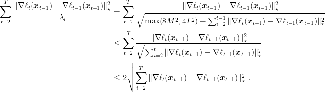
Focusing on the first term, for
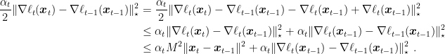
Choose 

For 

Now observe the assumption 


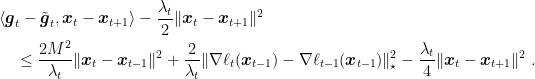
Putting all together, we have the first stated bound.
The second one is obtained observing that
Note that if the losses are all the same, the regret becomes a constant! This is not surprising, because the prediction of the next loss is a linear approximation of the previous loss. Indeed, looking back at the proof, the key idea is to use the smoothness to argue that, if even the past subgradient was taken in a different point than the current one, it is still a good prediction of the current subgradient.
Remark 2 Note that the assumption of smoothness is necessary. Indeed, passing always the same function and using online-to-batch conversion, would result in a convergence rate of
for a Lipschitz function, that is impossible.
3. History Bits
The Optimistic Online Mirror Descent algorithm was proposed by (Chiang, C.-K. and Yang, T. and Lee, C.-J. and Mahdavi, M. and Lu, C.-J. and Jin, R. and Zhu, S., 2012) and extended in (A. Rakhlin and K. Sridharan, 2013) to use arbitrary “hallucinated” losses. The Optimistic FTRL version was proposed in (A. Rakhlin and K. Sridharan, 2013) and rediscovered in (Steinhardt, J. and Liang, P., 2014), even if it was called Online Mirror Descent for the misnaming problem we already explained. The proof of Theorem 1 I present here is new.
Corollary 2 was proved by (Chiang, C.-K. and Yang, T. and Lee, C.-J. and Mahdavi, M. and Lu, C.-J. and Jin, R. and Zhu, S., 2012) for Optimistic OMD and presented in a similar form in (P. Joulani and A. György and C. Szepesvári, 2017) for Optimistic FTRL, but for bounded domains.

Thank you! How would you implement that? So what would the update rule be w_t+1 = ?
LikeLike
I added Example 1, I hope it helps to clarify how to implement Optimistic FTRL.
LikeLike