Saddle-Point Problems and OCO

12/4/2021: In the previous version of this post there were some incorrect details that didn’t allow me to sleep well at night. So, I rewrote it in the correct formalism, but please let me know if you see mistakes.

In this post, we talk about solving saddle-point problems with online convex optimization (OCO) algorithms. Next time, I’ll show the connection to two-person zero-sum games and boosting.

1. Saddle-Point Problems

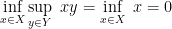
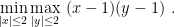
We want to solve the following saddle-point problem

$\displaystyle \label{eq:saddle_point} \inf_{{\boldsymbol x} \in X} \sup_{{\boldsymbol y}\in Y} \ f({\boldsymbol x},{\boldsymbol y})~. \ \ \ \ \ (1)$

Let’s say from the beginning that we need inf and sup rather than min and max because the minimum or maximum might not exist. Everytime we know for sure the inf/sup are attained, I’ll substitute them with min/max.

While for the minimization of functions is clear what it means to solve it, it might not be immediate to see what is the meaning of “solving” the saddle-point problem in (1). It turns out that the proper notion we are looking for is the one of saddle-point.

Definition 1. Let ${X \subseteq {\mathbb R}^n}$ , ${Y \subseteq {\mathbb R}^m}$ , and ${f: X \times Y \rightarrow {\mathbb R}}$ . A point ${({\boldsymbol x}^\star, {\boldsymbol y}^\star) \in X \times Y}$ is a saddle-point of ${f}$ in ${X\times Y}$ if

$\displaystyle f({\boldsymbol x}^\star, {\boldsymbol y}) \leq f({\boldsymbol x}^\star, {\boldsymbol y}^\star) \leq f({\boldsymbol x}, {\boldsymbol y}^\star), \quad \forall {\boldsymbol x} \in X, {\boldsymbol y} \in Y~.$

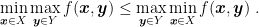
We will now state conditions under which there exists a saddle-point that solves (1). First, we need an easy lemma.

Lemma 2. Let ${f}$ is any function from a non-empty product set ${X \times Y}$ to ${{\mathbb R}}$ . Then,

$\displaystyle \inf_{{\boldsymbol x} \in X} \sup_{{\boldsymbol y} \in Y} \ f({\boldsymbol x},{\boldsymbol y}) \geq \sup_{{\boldsymbol y} \in Y} \inf_{{\boldsymbol x} \in X} \ f({\boldsymbol x},{\boldsymbol y})~.$

Proof: For any ${{\boldsymbol x}' \in X}$ and ${{\boldsymbol y} \in Y}$ we have that ${f({\boldsymbol x}',{\boldsymbol y}) \geq \inf_{{\boldsymbol x} \in X} \ f({\boldsymbol x},{\boldsymbol y})}$ . This implies that ${\sup_{{\boldsymbol y} \in Y} \ f({\boldsymbol x}', {\boldsymbol y}) \geq \sup_{{\boldsymbol y} \in Y} \inf_{{\boldsymbol x} \in X} \ f({\boldsymbol x},{\boldsymbol y})}$ for all ${{\boldsymbol x}' \in X}$ that gives the stated inequality. $\Box$

We can now state the following theorem.

Theorem 3. Let ${f}$ any function from a non-empty product set ${X \times Y}$ to ${{\mathbb R}}$ . A point ${({\boldsymbol x}^\star, {\boldsymbol y}^\star)}$ is a saddle-point of ${f}$ if and only if the supremum in

$\displaystyle \sup_{{\boldsymbol y} \in Y} \inf_{{\boldsymbol x} \in X} \ f({\boldsymbol x}, {\boldsymbol y})$

is attained at ${{\boldsymbol y}^\star}$ , the infimum in

$\displaystyle \inf_{{\boldsymbol x} \in X} \sup_{{\boldsymbol y} \in Y} \ f({\boldsymbol x}, {\boldsymbol y})$

is attained at ${{\boldsymbol x}^\star}$ , and these two expressions are equal.

Proof: If ${({\boldsymbol x}^\star,{\boldsymbol y}^\star)}$ is a saddle-point, then we have

$\displaystyle \begin{aligned} f({\boldsymbol x}^\star,{\boldsymbol y}^\star) &= \inf_{{\boldsymbol x} \in X} \ f({\boldsymbol x}, {\boldsymbol y}^\star) \leq \sup_{{\boldsymbol y} \in Y} \inf_{{\boldsymbol x} \in X} \ f({\boldsymbol x}, {\boldsymbol y})\\ f({\boldsymbol x}^\star,{\boldsymbol y}^\star) &= \sup_{{\boldsymbol y} \in Y} \ f({\boldsymbol x}^\star, {\boldsymbol y}) \geq \inf_{{\boldsymbol x} \in X} \sup_{{\boldsymbol y} \in Y} \ f({\boldsymbol x}, {\boldsymbol y})~. \end{aligned}$

From Lemma 2, we have that these quantities must be equal, so that the three conditions in the theorem are satisfied.

For the other direction, if the conditions are satisfied, then we have

$\displaystyle f({\boldsymbol x}^\star, {\boldsymbol y}^\star) \leq \sup_{{\boldsymbol y} \in Y} \ f({\boldsymbol x}^\star, {\boldsymbol y}) = \inf_{{\boldsymbol x} \in X} \ f({\boldsymbol x}, {\boldsymbol y}^\star) \leq f({\boldsymbol x}^\star, {\boldsymbol y}^\star)~.$

Hence, ${({\boldsymbol x}^\star,{\boldsymbol y}^\star)}$ is a saddle-point. $\Box$

Remark 1. The above theorem tells a surprising thing: If a saddle-point exists, then there might be multiple ones, and all of them must have the same minimax value. This might seem surprising, but it is due to the fact that the definition of saddle-point is a global and not a local property. Moreover, if the ${\inf\sup}$ and ${\sup\inf}$ problem have different values, no saddle-point exists.

Remark 2. Consider the case that the value of the ${\inf\sup}$ and ${\inf\sup}$ are different. If your favorite optimization procedure to find the solution of a saddle-point problem does not distinguish between a ${\inf\sup}$ and ${\sup\inf}$ formulation, then it cannot be correct!

Let’s show a couple of examples that show that the conditions above are indeed necessary.

no_saddle_point — Figure 1. ${f(x,y)=(x-y)^2}$ does not have a saddle point.

Figure 1. ${f(x,y)=(x-y)^2}$ does not have a saddle point.

Example 1. Let ${f(x,y)=(x-y)^2}$ , ${X=[-1,1]}$ , and ${Y=[-1,1]}$ . Then, we have

$\displaystyle \inf_{x \in X} \sup_{y \in Y} \ (x-y)^2 = \inf_{x \in X} \ (1+|x|)^2 = 1,$

while

$\displaystyle \sup_{y \in Y} \inf_{x \in X} \ (x-y)^2 = \sup_{y \in Y} 0 = 0~.$

Indeed, from Figure 1 we can see that there is no saddle-point.

Example 2. Let ${f(x,y)=x y }$ , ${X=(0,1]}$ , and ${Y=(0,1]}$ . Then, we have

$\displaystyle \inf_{x \in X} \sup_{y \in Y} \ x y = \inf_{x \in X} \ x = 0$

and

$\displaystyle \sup_{y \in Y} \inf_{x \in X} \ xy = 0~.$

Here, even if inf sup is equal to sup inf, the saddle-point does not exist because the inf in the first expression is not attained in a point of ${X}$ .

This theorem also tells us that in order to find a saddle-point of a function ${f}$ , we need to find the minimizer in ${{\boldsymbol x}}$ of ${\sup_{{\boldsymbol y} \in Y} \ f({\boldsymbol x},{\boldsymbol y})}$ and the maximizer in ${y}$ of ${\inf_{{\boldsymbol x} \in X} \ f({\boldsymbol x},{\boldsymbol y})}$ . Let’s now use this knowledge to design a proper measure of progress towards the saddle-point.

We might be tempted to use ${f({\boldsymbol x}', {\boldsymbol y}')-f({\boldsymbol x}^\star,{\boldsymbol y}^\star)}$ as a measure of suboptimality of ${({\boldsymbol x}',{\boldsymbol y}')}$ with respect to the saddle-point ${({\boldsymbol x}^\star,{\boldsymbol y}^\star)}$ . Unfortunately, this quantity can be negative or equal to zero for an infinite number of points ${({\boldsymbol x}',{\boldsymbol y}')}$ that are not saddle-points. We might then think to use some notion of distance to the saddle-point, like ${\|{\boldsymbol x}'-{\boldsymbol x}^\star\|^2_2+\|{\boldsymbol y}'-{\boldsymbol y}^\star\|^2_2}$ , but this quantity in general can go to zero at an arbitrarily slow rate. To see why consider the case that ${f({\boldsymbol x},{\boldsymbol y})=h({\boldsymbol x})}$ , so that the saddle-point problem reduces to minimize a convex function. So, assuming only convexity, the rate of convergence to a minimizer of ${f}$ can be arbitrarily slow. Hence, we need something different.

Observe that the Theorem 3 says one of the problems we should solve is

$\displaystyle \inf_{{\boldsymbol x} \in X} \ h({\boldsymbol x}),$

where ${h({\boldsymbol x}) = \sup_{{\boldsymbol y}\in Y} \ f({\boldsymbol x},{\boldsymbol y})}$ . In this view, the problem looks like a standard convex optimization problem, where the objective function has a particular structure. Moreover, in this view we only focus on the variables ${{\boldsymbol x}}$ . The standard measure of convergence in this case for a point ${{\boldsymbol x}'}$ , the suboptimality gap, can be written as

$\displaystyle h({\boldsymbol x}') - \inf_{{\boldsymbol x} \in X} h({\boldsymbol x}) = \sup_{{\boldsymbol y}\in Y} \ f({\boldsymbol x}',{\boldsymbol y}) - \inf_{{\boldsymbol x} \in X} \sup_{{\boldsymbol y}\in Y} \ f({\boldsymbol x},{\boldsymbol y})~.$

We also have to find the maximizer in ${y}$ of ${\inf_{{\boldsymbol x} \in X} \ f({\boldsymbol x},{\boldsymbol y})}$ , hence we have

$\displaystyle \sup_{{\boldsymbol y} \in Y} \ g({\boldsymbol y}),$

where ${g({\boldsymbol y}) = \inf_{{\boldsymbol x}\in X} \ f({\boldsymbol x},{\boldsymbol y})}$ . This also implies another measure of convergence in which we focus only on the variable ${{\boldsymbol y}}$ :

$\displaystyle \sup_{{\boldsymbol y} \in Y} \ g({\boldsymbol y}) - g({\boldsymbol y}') = \sup_{{\boldsymbol y}\in Y} \inf_{{\boldsymbol x} \in X} \ f({\boldsymbol x},{\boldsymbol y}) - \inf_{{\boldsymbol x}\in X} \ f({\boldsymbol x},{\boldsymbol y}') ~.$

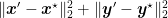
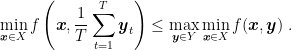
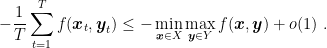
Finally, in case we are interested in studying the quality of a joint solution ${({\boldsymbol x}',{\boldsymbol y}')}$ , a natural measure is a sum of the two measures above:

$\displaystyle \sup_{{\boldsymbol y}\in Y} \ f({\boldsymbol x}',{\boldsymbol y}) - \inf_{{\boldsymbol x} \in X} \sup_{{\boldsymbol y}\in Y} \ f({\boldsymbol x},{\boldsymbol y}) + \sup_{{\boldsymbol y}\in Y} \inf_{{\boldsymbol x} \in X} \ f({\boldsymbol x},{\boldsymbol y}) - \inf_{{\boldsymbol x}\in X} \ f({\boldsymbol x},{\boldsymbol y}') = \sup_{{\boldsymbol y}\in Y} \ f({\boldsymbol x}',{\boldsymbol y}) - \inf_{{\boldsymbol x} \in X} \ f({\boldsymbol x}, {\boldsymbol y}'),$

where we assumed the existence of a saddle-point to say that ${\inf_{{\boldsymbol x} \in X} \sup_{{\boldsymbol y}\in Y} \ f({\boldsymbol x},{\boldsymbol y}) = \sup_{{\boldsymbol y}\in Y} \inf_{{\boldsymbol x} \in X} \ f({\boldsymbol x},{\boldsymbol y})}$ from Theorem 3. This measure is called duality gap. From the definition it should be clear that the duality gap is always non-negative. Let’s add even more intuition of the duality gap definition, using the one of ${\epsilon}$ -saddle-point.

Definition 4. Let ${X \subseteq {\mathbb R}^n}$ , ${Y \subseteq {\mathbb R}^m}$ , and ${f: X \times Y \rightarrow {\mathbb R}}$ . A point ${({\boldsymbol x}^\star, {\boldsymbol y}^\star) \in X \times Y}$ is a ${\epsilon}$ -saddle-point of ${f}$ in ${X\times Y}$ if

$\displaystyle f({\boldsymbol x}^\star,{\boldsymbol y}) -\epsilon \leq f({\boldsymbol x}^\star,{\boldsymbol y}^\star) \leq f({\boldsymbol x},{\boldsymbol y}^\star) + \epsilon, \quad \forall {\boldsymbol x} \in X, {\boldsymbol y} \in Y~.$

This definition is useful because we cannot expect to numerically calculate a saddle-point with infinite precision, but we can be find something that satisfies the saddle-point definition up to a ${\epsilon}$ . Obviously, any saddle-point is also an ${\epsilon}$ -saddle-point.

Now, the notion of ${\epsilon}$ -saddle-point is equivalent up to a multiplicative constant to the ${\epsilon}$ duality gap. In fact, it is easy to see that if ${({\boldsymbol x}^\star,{\boldsymbol y}^\star)}$ is an ${\epsilon}$ -saddle-point then its duality gap of ${2\epsilon}$ . In turn, a duality gap of ${2 \epsilon}$ and the existence of a saddle-point imply that the point is a ${2\epsilon}$ -saddle.

The above reasoning told us that finding the saddle-point of the function ${f}$ is equivalent to solving a maximization problem and a minimization problem. However, is it always the case that the saddle-point exists? So, let’s now move to easily checkable sufficient conditions for the existence of saddle-point. For this, we can state the following theorem.

Theorem 5. Let ${X}$ , ${Y}$ be compact convex subsets of ${{\mathbb R}^n}$ and ${{\mathbb R}^m}$ respectively. Let ${f : X \times Y \rightarrow {\mathbb R}}$ a continuous function, convex in its first argument, and concave in its second. Then, we have that

$\displaystyle \min_{{\boldsymbol x} \in X} \max_{{\boldsymbol y}\in Y} \ f({\boldsymbol x},{\boldsymbol y}) = \max_{{\boldsymbol y}\in Y} \min_{{\boldsymbol x} \in X} \ f({\boldsymbol x},{\boldsymbol y})~.$

This theorem gives us sufficient conditions to have the min-max problem equal to the max-min one. So, for example, thanks to the Weierstrass theorem, the assumptions in Theorem 5, in light of Theorem 3, are sufficient conditions for the existence of a saddle-point.

We defer the proof of this theorem for a bit and we now turn ways to solve the saddle-point problem in (1).

2. Solving Saddle-Point Problems with OCO

Let’s show how to use Online Convex Optimization (OCO) algorithms to solve saddle-point problems.

algo_spp_1

Suppose to use an OCO algorithm fed with losses ${\ell_t({\boldsymbol x})= f({\boldsymbol x},{\boldsymbol y}_t)}$ that produces the iterates ${{\boldsymbol x}_t}$ and another OCO algorithm fed with losses ${h_t({\boldsymbol y})=-f({\boldsymbol x}_t,{\boldsymbol y})}$ that produces the iterates ${{\boldsymbol y}_t}$ . Then, we can state the following Theorem.

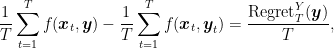
Theorem 6. Let ${f:X\times Y\rightarrow {\mathbb R}}$ be convex in the first argument and concave in the second. Then, with the notation in Algorithm 2, for any ${{\boldsymbol x} \in X}$ , we have

$\displaystyle \frac{1}{T}\sum_{t=1}^T f({\boldsymbol x}_t, {\boldsymbol y}_t) - \frac{1}{T}\sum_{t=1}^T f({\boldsymbol x},{\boldsymbol y}_t) = \frac{\text{Regret}^{X}_T({\boldsymbol x})}{T},$

where ${\text{Regret}^{X}_T({\boldsymbol x})=\sum_{t=1}^T \ell_t({\boldsymbol x}_t) - \sum_{t=1}^T \ell_t({\boldsymbol x})}$ .

For any ${{\boldsymbol y} \in Y}$ , we have

$\displaystyle \frac{1}{T}\sum_{t=1}^T f({\boldsymbol x}_t,{\boldsymbol y}) - \frac{1}{T}\sum_{t=1}^T f({\boldsymbol x}_t, {\boldsymbol y}_t) = \frac{\text{Regret}^{Y}_T({\boldsymbol y})}{T},$

where ${\text{Regret}^{Y}_T({\boldsymbol y})=\sum_{t=1}^T h_t({\boldsymbol y}_t) - \sum_{t=1}^{T} h_t({\boldsymbol y})}$ .

Also, if ${f}$ is continuous and ${X}$ , ${Y}$ compact, we have

$\displaystyle \max_{{\boldsymbol y}\in Y} f(\bar{{\boldsymbol x}}_T, {\boldsymbol y}) - \min_{{\boldsymbol x}\in X} f({\boldsymbol x},\bar{{\boldsymbol y}}_T) \leq \frac{\text{Regret}^{X}_T({\boldsymbol x}'_T)+\text{Regret}^{Y}_T({\boldsymbol y}'_T)}{T},$

for any ${{\boldsymbol x}_T'\in\arg\min_{{\boldsymbol x}\in X}f({\boldsymbol x},\bar{{\boldsymbol y}}_T)}$ and ${{\boldsymbol y}_T'\in\arg\max_{{\boldsymbol y}\in Y}f(\bar{{\boldsymbol x}}_T,{\boldsymbol y})}$ .

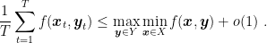
Proof: The first two equalities are obtained simply observing that ${\ell_t({\boldsymbol x})=f({\boldsymbol x},{\boldsymbol y}_t)}$ and ${h_t({\boldsymbol y})=-f({\boldsymbol x}_t,{\boldsymbol y})}$ .

For the inequality, using Jensen’s inequality, we obtain

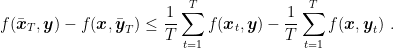
$\displaystyle \begin{aligned} f(\bar{{\boldsymbol x}}_T,{\boldsymbol y})- f({\boldsymbol x},\bar{{\boldsymbol y}}_T) &\leq \frac{1}{T}\sum_{t=1}^{T}f({\boldsymbol x}_t,{\boldsymbol y})- \frac{1}{T} \sum_{t=1}^{T}f({\boldsymbol x},{\boldsymbol y}_t)~. \end{aligned}$

Summing the first two equalities, using the above inequality, and taking ${{\boldsymbol x}={\boldsymbol x}'_T\in\arg\min_{{\boldsymbol x}\in\mathcal{X}} f({\boldsymbol x},\bar{{\boldsymbol y}}_T)}$ and ${{\boldsymbol y}={\boldsymbol y}'_T\in\arg\max_{{\boldsymbol y}\in\mathcal{Y}} f(\bar{{\boldsymbol x}}_T,{\boldsymbol y})}$ , we get the stated inequality. $\Box$

From this theorem, we can immediately prove the following corollary.

Corollary 7. Let ${f:X\times Y\rightarrow {\mathbb R}}$ be continuous, convex in the first argument, and concave in the second. Assume that ${X}$ and ${Y}$ are compact and that the ${X}$ -player and ${Y}$ -player use no-regret algorithms, possibly different, than

$\displaystyle \lim_{T\rightarrow\infty}\max_{{\boldsymbol y}\in\mathcal{Y}} f(\bar{{\boldsymbol x}}_T, {\boldsymbol y}) - \min_{{\boldsymbol x}\in\mathcal{X}} f({\boldsymbol x},\bar{{\boldsymbol y}}_T)=0~.$

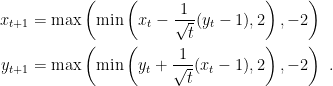
Example 3. Consider the saddle-point problem

$\displaystyle \min_{|x|\leq 2} \max_{|y|\leq 2} \ (x-1) (y-1)~.$

The saddle-point of this problem is ${(x,y)=(1,1)}$ . We can find it using, for example, Projected Online Gradient Descent. So, setting ${{\boldsymbol x}_1={\boldsymbol y}_1=0}$ , we have the iterations

$\displaystyle \begin{aligned} x_{t+1} &= \max\left(\min\left(x_t - \frac{1}{\sqrt{t}} (y_t-1),2\right),-2\right)\\ y_{t+1} &= \max\left(\min\left(y_t + \frac{1}{\sqrt{t}} (x_t-1),2\right),-2\right)~. \end{aligned}$

According to Theorem 6, the duality gap in ${(\frac1T \sum_{t=1}^T x_t, \frac1T \sum_{t=1}^T y_t)}$ converges to 0.

Surprisingly, we can even prove a (simpler version of the) minimax theorem from the above result! In particular, we will use the additional assumption that there exist OCO algorithms that minimize ${\ell_t}$ and ${h_t}$ have sublinear regret.
Proof with OCO assumption: From Lemma 2, we have one inequality. Hence, we now have to prove the other inequality.

We will use a constructive proof. Let’s use Algorithm 2 and Theorem 6. For the first player, for any ${{\boldsymbol x} \in X}$ we have

$\displaystyle \frac{1}{T}\sum_{t=1}^T f({\boldsymbol x}_t, {\boldsymbol y}_t) = \frac{1}{T}\sum_{t=1}^T f({\boldsymbol x},{\boldsymbol y}_t) + \frac{\text{Regret}^{X}_T({\boldsymbol x})}{T} \leq f\left({\boldsymbol x},\frac{1}{T}\sum_{t=1}^T {\boldsymbol y}_t\right) + \frac{\text{Regret}^{X}_T({\boldsymbol x})}{T}~.$

Observe that

$\displaystyle \min_{{\boldsymbol x} \in X} f\left({\boldsymbol x},\frac{1}{T}\sum_{t=1}^T {\boldsymbol y}_t\right) \leq \max_{{\boldsymbol y} \in Y} \min_{{\boldsymbol x} \in X} f({\boldsymbol x},{\boldsymbol y})~.$

Hence, using an OCO algorithm that has ${o(T)}$ regret for each ${{\boldsymbol x} \in X}$ , we have

$\displaystyle \frac{1}{T}\sum_{t=1}^T f({\boldsymbol x}_t, {\boldsymbol y}_t) \leq \max_{{\boldsymbol y} \in Y} \min_{{\boldsymbol x} \in X} f({\boldsymbol x},{\boldsymbol y})+o(1)~.$

In the same way, we have

$\displaystyle -\frac{1}{T}\sum_{t=1}^T f({\boldsymbol x}_t, {\boldsymbol y}_t) \leq -\min_{{\boldsymbol x} \in X} \max_{{\boldsymbol y} \in Y} f({\boldsymbol x},{\boldsymbol y})+o(1)~.$

Summing the two inequalities, taking ${T\rightarrow \infty}$ , and using the sublinear regret assumption, we have

$\displaystyle \min_{{\boldsymbol x} \in X} \max_{{\boldsymbol y} \in Y} f({\boldsymbol x},{\boldsymbol y}) \leq \max_{{\boldsymbol y} \in Y} \min_{{\boldsymbol x} \in X} f({\boldsymbol x},{\boldsymbol y})~.$

$\Box$

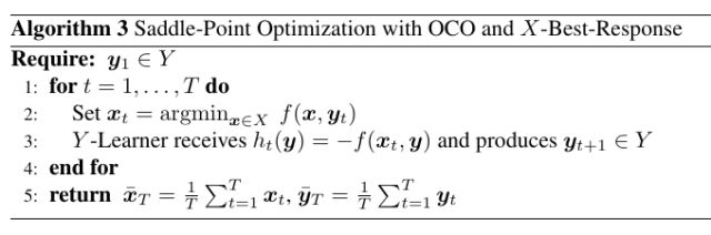
2.1. Variations with Best Response and Alternation

In some cases, it is easy to compute the max with respect to ${{\boldsymbol y} \in Y}$ of ${f({\boldsymbol x}_t,{\boldsymbol y})}$ for a given ${{\boldsymbol x}_t}$ . For example, this is trivial for bilinear games over the simplex. In these cases, we can remove the second learner and just use its best response in each round. Note that in this way we are making one of the two players “stronger” through the knowledge of the loss of the next round. However, this is perfectly fine: The proof in Theorem 6 is still perfectly valid.

algo_spp_2

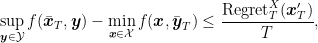
In this case, the ${Y}$ -player has an easy life: it knows the loss before making the prediction, hence it can just output the minimizer of the loss in ${Y}$ . Hence, we also have that the regret of the ${Y}$ -player will be non-positive and it will not show up in Theorem 6. Putting all together, we can state the following corollary.

Corollary 8. Let ${f:X\times Y\rightarrow {\mathbb R}}$ be continuous, convex in the first argument, and concave in the second. Assume ${X}$ compact and that the argmax of the ${Y}$ -player is never empty. Then, with the notation in Algorithm 2, we have

$\displaystyle \sup_{{\boldsymbol y}\in\mathcal{Y}} f(\bar{{\boldsymbol x}}_T, {\boldsymbol y}) - \min_{{\boldsymbol x}\in\mathcal{X}} f({\boldsymbol x},\bar{{\boldsymbol y}}_T) \leq \frac{\text{Regret}^{X}_T({\boldsymbol x}'_T)}{T},$

for any ${{\boldsymbol x}_T'\in\arg\min_{{\boldsymbol x}\in X}f({\boldsymbol x},\bar{{\boldsymbol y}}_T)}$ and where ${\text{Regret}^{X}_T({\boldsymbol x})=\sum_{t=1}^T \ell_t({\boldsymbol x}_t) - \sum_{t=1}^{T} \ell_t({\boldsymbol x})}$ .

This alternative seems interesting from a theoretical point of view because it allows to avoid the complexity of learning in the ${Y}$ space, for example removing the dependency on its dimension. Of course, an analogous result can be stated using best-response for the ${X}$ -player and an OCO algorithm for the ${Y}$ -player.

algo_spp_3

There is a third variant, very used in empirical implementations, especially of Counterfactual Regret Minimization (CFR) (Zinkevich et al., 2007). It is called alternation and it breaks the simultaneous reveal of the actions of the two players. Instead, we use the updated prediction of the first player to construct the loss of the second player. Empirically, this variant seems to greatly speed-up the convergence of the duality gap.

algo_spp_4

For this version, Theorem 6 does not hold anymore because the terms ${f({\boldsymbol x}_t,{\boldsymbol y}_t)}$ and ${f({\boldsymbol x}_{t+1},{\boldsymbol y}_t)}$ are now different, however we can prove a similar guarantee.

Theorem 9. Let ${f:X\times Y\rightarrow {\mathbb R}}$ continuous, convex in the first argument, and concave in the second. Assume that ${X}$ and ${Y}$ are compact. Then, with the notation in Algorithm 4, for any ${{\boldsymbol x}_T'\in\arg\min_{{\boldsymbol x}\in\mathcal{X}}f({\boldsymbol x},\bar{{\boldsymbol y}}_T)}$ and any ${{\boldsymbol y}_T'\in\arg\max_{{\boldsymbol y}\in\mathcal{Y}}f(\bar{{\boldsymbol x}}_T,{\boldsymbol y})}$ we have

$\displaystyle \max_{{\boldsymbol y}\in\mathcal{Y}} f(\bar{{\boldsymbol x}}_T, {\boldsymbol y}) - \min_{{\boldsymbol x}\in\mathcal{X}} f({\boldsymbol x},\bar{{\boldsymbol y}}_T) \leq \frac{\text{Regret}^{X}_T({\boldsymbol x}'_T)+\text{Regret}^{Y}_T({\boldsymbol y}'_T)+\sum_{t=1}^{T} (f({\boldsymbol x}_{t+1},{\boldsymbol y}_t)-f({\boldsymbol x}_{t},{\boldsymbol y}_t))}{T},$

where ${\text{Regret}^{Y}_T({\boldsymbol y})=\sum_{t=1}^T h_t({\boldsymbol y}_t) - \sum_{t=1}^{T} h_t({\boldsymbol y})}$ and ${\text{Regret}^{X}_T({\boldsymbol x})=\sum_{t=1}^T \ell_t({\boldsymbol x}_t) - \sum_{t=1}^T \ell_t({\boldsymbol x})}$ .

Proof: Note that ${\ell_t({\boldsymbol x})=f({\boldsymbol x},{\boldsymbol y}_t)}$ , and ${h_t({\boldsymbol y})=-f({\boldsymbol x}_{t+1},{\boldsymbol y})}$ . By Jensen’s inequality, we have

$\displaystyle \begin{aligned} T(f(\bar{{\boldsymbol x}}_T, {\boldsymbol y}) - f({\boldsymbol x},\bar{{\boldsymbol y}}_T)) &\leq \sum_{t=1}^{T}f({\boldsymbol x}_{t+1},{\boldsymbol y})- \sum_{t=1}^{T}f({\boldsymbol x},{\boldsymbol y}_t)\\ &=\sum_{t=1}^{T}f({\boldsymbol x}_{t+1},{\boldsymbol y})-\sum_{t=1}^{T}f({\boldsymbol x}_{t+1},{\boldsymbol y}_t) +\sum_{t=1}^{T}f({\boldsymbol x}_{t},{\boldsymbol y}_t)-\sum_{t=1}^{T}f({\boldsymbol x},{\boldsymbol y}_t)\\ &\quad +\sum_{t=1}^{T}f({\boldsymbol x}_{t+1},{\boldsymbol y}_t)-\sum_{t=1}^{T}f({\boldsymbol x}_{t},{\boldsymbol y}_t)\\ &= \sum_{t=1}^{T} (h_t({\boldsymbol y}_t)-h_t({\boldsymbol y}))+\sum_{t=1}^{T}(\ell_t({\boldsymbol x}_t)-\ell_t({\boldsymbol x})) + \sum_{t=1}^{T} (f({\boldsymbol x}_{t+1},{\boldsymbol y}_t)-f({\boldsymbol x}_{t},{\boldsymbol y}_t))~. \end{aligned}$

Taking ${{\boldsymbol x}={\boldsymbol x}'_T\in\arg\min_{{\boldsymbol x}\in\mathcal{X}} f({\boldsymbol x},\bar{{\boldsymbol y}}_T)}$ and ${{\boldsymbol y}={\boldsymbol y}'_T\in\arg\max_{{\boldsymbol y}\in\mathcal{Y}} f(\bar{{\boldsymbol x}}_T,{\boldsymbol y})}$ , we get the stated result. $\Box$

Remark 3. In the case that ${f(\cdot,\cdot)}$ is linear in the first argument, using OMD for the ${X}$ -player we have that ${f({\boldsymbol x}_t,{\boldsymbol y}_t) = \ell_t({\boldsymbol x}_t) \geq \ell_t({\boldsymbol x}_{t+1})=f({\boldsymbol x}_{t+1},{\boldsymbol y}_t)}$ . Hence, in this case the additional term in Theorem 9 is negative, showing a (marginal) improvement to the convergence rate.

Next post, we will show how to connect saddle-point problems with Game Theory.

3. History Bits

Theorem 3 is (Rockafellar, 1970, Lemma 36.2).

The proof of Theorem 6 is from (Liu and Orabona, 2021) and it is a minor variation on the one in (Abernethy and Wang, 2017): (Liu and Orabona, 2021) stressed the dependency of the regret on a competitor that can be useful for refined bounds, as we will show next time for Boosting. It is my understanding that different variant of this theorem are known in the game theory community as “Folk Theorems”, because such result was widely known among game theorists in the 1950s, even though no one had published it.

The celebrated minimax theorem for zero-sum two-person games was first discovered by John von Neumann in the 1920s (von Neumann, 1928)(von Neumann and Morgenstern, 1944). The version is state here is a simplification of the generalization due to (Sion, 1958). The proof here is from (Abernethy and Wang, 2017). A similar proof is in (Cesa-Bianchi and Lugosi, 2006) based on a discretization of the space that in turn is based on the one in (Freund, Y. and Schapire, 1996)(Freund, Y. and Schapire, 1999).

Algorithms 2 and 3 are a generalization of the algorithm for boosting in (Freund and Schapire, 1996)(Freund and Schapire, 1999). Algorithm 2 was also used in (Abernethy and Wang, 2017) to recover variants of the Frank-Wolfe algorithm (Frank and Wolfe, 1956).

It is not clear who invented alternation. Christian Kroer told me that it was a known trick used in implementations of CFR for the computer poker competition from 2010 or so. Note that in CFR the method of choice is Regret Matching (Hart and Mas-Colell, 2000). However, (Kroer, 2020) empirically shows that alternation improves a lot even OGD for solving bilinear games. (Tammelin et al., 2015) explicitly include this trick in their implementation of an improved version of CFR called CFR+, claiming that it would still guarantee convergence. However, (Farina et al., 2019) pointed out that averaging of the iterates in alternation might not produce a solution to the min-max problem, providing a counterexample. Theorem 9 is from (Burch et al., 2019) (see also (Kroer, 2020)).

There is also a complementary view on alternation: (Zhang et al., 2021) link alternating updates to Gauss-Seidel methods in numerical linear algebra, in contrast to the simultaneous updates of the Jacobi method. Also, they provide a good review of the optimization literature on the advantages of alternation, but this paper and the papers they cite do not seem to be aware of the use of alternation in CFR.

Acknowledgements

Thanks to Christian Kroer for the history of alternation in CFR, and to Gergely Neu for the references on alternation in the optimization community. Thanks to Nicolò Campolongo for hunting down my typos. Also, thanks to Christian Kroer for his great lecture notes that helped me getting started on this topic.

Pingback: Saddle-Points, Game Theory, and Boosting – Parameter-free Learning and Optimization Algorithms
Pingback: A Simple Proof for Optimistic OMD – Parameter-free Learning and Optimization Algorithms
Pingback: Saddle-Point Optimization With Optimism – Parameter-free Learning and Optimization Algorithms

Share this:

Like this:

Related

Leave a Reply Cancel reply