Adaptive Algorithms: L* bounds and AdaGrad

This post is part of the lecture notes of my class “Introduction to Online Learning” at Boston University, Fall 2019.

You can find all the lectures I published here.

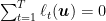
In this lecture, we will explore a bit more under which conditions we can get better regret upper bounds than ${O(D L \sqrt{T})}$ . Also, we will obtain this improved guarantees in an automatic way. That is, the algorithm will be adaptive to characteristics of the sequence of loss functions, without having to rely on information about the future.

1. Adaptive Learning Rates for Online Subgradient Descent

Consider the minimization of the linear regret

$\displaystyle \text{Regret}_T({\boldsymbol u})=\sum_{t=1}^T \langle {\boldsymbol g}_t, {\boldsymbol x}_t\rangle - \sum_{t=1}^T \langle {\boldsymbol g}_t, {\boldsymbol u}\rangle$

Using Online Subgradient Descent (OSD), we said that the regret for bounded domains can be upper bounded by

$\displaystyle \sum_{t=1}^T \langle {\boldsymbol g}_t, {\boldsymbol x}_t\rangle - \sum_{t=1}^T \langle {\boldsymbol g}_t, {\boldsymbol u}\rangle \leq \frac{D^2}{2 \eta_T} + \frac{1}{2}\sum_{t=1}^T \eta_t \|{\boldsymbol g}_t\|_2^2~.$

With a fixed learning rate, the learning rate that minimizes this upper bound on the regret is

$\displaystyle \eta^\star_T = \frac{D}{\sqrt{\sum_{t=1}^T \|g_t\|_2^2}}~.$

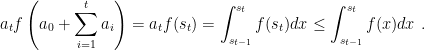
Unfortunately, as we said, this learning rate cannot be used because it assumes the knowledge of the future rounds. However, we might be lucky and we might try to just approximate it in each round using the knowledge up to time ${t}$ . That is, we might try to use

$\displaystyle \label{eq:ada_eta} \eta_t = \frac{D}{\sqrt{\sum_{i=1}^t \|{\boldsymbol g}_i\|_2^2}}~. \ \ \ \ \ (1)$

Observe that ${\eta_T=\eta_T^\star}$ , so the first term of the regret would be exactly what we need! For the other term, the optimal learning rate would give us

$\displaystyle \frac{1}{2}\sum_{t=1}^T \eta_T^\star \|{\boldsymbol g}_t\|_2^2 = \frac{1}{2} D \sqrt{\sum_{t=1}^T \|{\boldsymbol g}_t\|_2^2}~.$

Now let’s see what we obtain with our approximation.

$\displaystyle \frac{1}{2}\sum_{t=1}^T \eta_t \|{\boldsymbol g}_t\|^2 = \frac{1}{2} D \sum_{t=1}^T \frac{\|{\boldsymbol g}_t\|_2^2}{\sqrt{\sum_{i=1}^t \|{\boldsymbol g}_i\|_2^2}}~.$

We need a way to upper bound that sum. The way to treat these sums, as we did in other cases, is to try to approximate them with integrals. So, we can use the following very handy Lemma that generalizes a lot of similar specific ones.

Lemma 1 Let ${a_0\geq 0}$ and ${f:[0,+\infty)\rightarrow [0, +\infty)}$ a nonincreasing function. Then

$\displaystyle \begin{aligned} \sum_{t=1}^T a_t f\left(a_0+\sum_{i=1}^{t} a_i\right) &\leq \int_{a_0}^{\sum_{t=0}^T a_t} f(x) dx~. \end{aligned}$

Proof: Denote by ${s_t=\sum_{i=0}^{t} a_i}$ .

$\displaystyle \begin{aligned} a_t f\left(a_0+ \sum_{i=1}^{t} a_i\right) = a_t f(s_t) = \int_{s_{t-1}}^{s_t} f(s_t) d x \leq \int_{s_{t-1}}^{s_t} f(x) d x~. \end{aligned}$

Summing over ${t=1, \cdots, T}$ , we have the stated bound. $\Box$

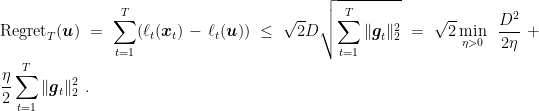
Using this Lemma, we have that

$\displaystyle \frac{1}{2} D \sum_{t=1}^T \frac{\|{\boldsymbol g}_t\|_2^2}{\sqrt{\sum_{i=1}^t \|{\boldsymbol g}_i\|_2^2}} \leq D \sqrt{\sum_{t=1}^T \|{\boldsymbol g}_t\|_2^2}~.$

Surprisingly, this term is only a factor of 2 worse than what we would have got from the optimal choice of ${\eta^\star_T}$ . However, this learning rate can be computed without knowledge of the future and it can actually be used! Overall, with this choice we get

$\displaystyle \label{eq:ada_grad_norm} \text{Regret}_T({\boldsymbol u}) =\sum_{t=1}^T \ell_t({\boldsymbol x}_t) - \sum_{t=1}^T \ell_t({\boldsymbol u}) \leq \frac32 D \sqrt{\sum_{t=1}^T \|{\boldsymbol g}_{t}\|_2^2}~. \ \ \ \ \ (2)$

Note that it is possible improve the constant in front of the bound to ${\sqrt{2}}$ by multiplying the learning rates by ${\frac{\sqrt{2}}{2}}$ . So, putting all together we have the following theorem.

Theorem 2 Let ${V\subseteq {\mathbb R}^d}$ a closed non-empty convex set with diameter ${D}$ , i.e. ${\max_{{\boldsymbol x},{\boldsymbol y}\in V} \|{\boldsymbol x}-{\boldsymbol y}\|_2 \leq D}$ . Let ${\ell_1, \cdots, \ell_T}$ an arbitrary sequence of convex functions ${\ell_t:{\mathbb R}^d \rightarrow (-\infty, +\infty]}$ subdifferentiable in open sets containing ${V}$ for ${t=1, \dots,T}$ . Pick any ${{\boldsymbol x}_1 \in V}$ and ${\eta_{t}=\frac{\sqrt{2}D}{2\sqrt{\sum_{i=1}^t \|{\boldsymbol g}_i\|_2^2}}, \ t=1, \dots, T}$ . Then, ${\forall {\boldsymbol u} \in V}$ , the following regret bound holds

$\displaystyle \text{Regret}_T({\boldsymbol u}) =\sum_{t=1}^T (\ell_t({\boldsymbol x}_t) - \ell_t({\boldsymbol u})) \leq \sqrt{2} D \sqrt{\sum_{t=1}^T \|{\boldsymbol g}_{t}\|_2^2} = \sqrt{2} \min_{\eta>0}\ \frac{D^2}{2\eta} + \frac{\eta}{2}\sum_{t=1}^T \|{\boldsymbol g}_t\|_2^2~.$

The second equality in the theorem clearly show the advantage of this learning rates: We obtain (almost) the same guarantee we would have got knowing the future gradients!

This is an interesting result on its own: it gives a principled way to set the learning rates with an almost optimal guarantee. However, there are also other consequences of this simple regret. First, we will specialize this result to the case that the losses are smooth.

2. Convex Analysis Bits: Smooth functions

We now consider a family of loss functions that have the characteristic of being lower bounded by the squared norm of the subgradient. We will also introduce the concept of dual norms. While dual norms are not strictly needed for this lecture, they give more generality and at the same time they allows me to slowly introduce some of the concepts that will be needed for the lectures on Online Mirror Descent.

Definition 3 The dual norm ${\|\cdot\|_\star}$ of a norm ${\|\cdot\|}$ is defined as ${\|{\boldsymbol \theta}\|_\star=\max_{{\boldsymbol x}: \|{\boldsymbol x}\|\leq 1} \ \langle {\boldsymbol \theta}, {\boldsymbol x}\rangle}$ .

Example 1 The dual norm of the L2 norm is the L2 norm. Indeed, ${\|{\boldsymbol \theta}\|_\star=\max_{{\boldsymbol x}: \|{\boldsymbol x}\|_2\leq 1} \ \langle {\boldsymbol \theta}, {\boldsymbol x}\rangle \leq \|{\boldsymbol \theta}\|_2}$ by Cauchy-Schwartz inequality. Also, set ${{\boldsymbol v}=\frac{{\boldsymbol \theta}}{\|{\boldsymbol \theta}\|_2}}$ , so ${\max_{{\boldsymbol x}: \|{\boldsymbol x}\|_2\leq 1} \ \langle {\boldsymbol \theta}, {\boldsymbol x}\rangle \geq \langle {\boldsymbol \theta}, {\boldsymbol v}\rangle = \|{\boldsymbol \theta}\|_2}$ .

If you never saw it before, the concept of dual norm can be a bit weird at first. One way to understand it is that it is a way to measure how “big” are linear functionals. For example, consider the linear function ${f({\boldsymbol x})=\langle {\boldsymbol z},{\boldsymbol x}\rangle}$ , we want to try to understand how big it is. So, we can measure ${\max_{{\boldsymbol x}\neq 0}\frac{\langle {\boldsymbol z},{\boldsymbol x}\rangle}{\|{\boldsymbol x}\|}}$ that is we measure how big is the output of the linear function compared to its input ${{\boldsymbol x}}$ , where ${{\boldsymbol x}}$ is measured with some norm. Now, you can show that the above is equivalent to the dual norm of ${{\boldsymbol z}}$ .

Remark 1 The definition of dual norm immediately implies ${\langle {\boldsymbol \theta}, {\boldsymbol x}\rangle \leq \|{\boldsymbol \theta}\|_\star \|{\boldsymbol x}\|}$ .

Now we can introduce smooth functions, using the dual norms defined above.

Definition 4 Let ${f:V \rightarrow {\mathbb R}}$ differentiable. We say that ${f}$ is ${M}$ -smooth w.r.t. ${\|\cdot\|}$ if ${\|\nabla f({\boldsymbol x}) -\nabla f({\boldsymbol y})\|_\star \leq M \|{\boldsymbol x}-{\boldsymbol y}\|}$ for all ${{\boldsymbol x}, {\boldsymbol y} \in V}$ .

Keeping in mind the intuition above on dual norms, taking the dual norm of a gradient makes sense if you associate each gradient with the linear functional ${\langle \nabla f({\boldsymbol x}), {\boldsymbol x}\rangle}$ , that is the one needed to create linear approximation of ${f}$ in ${{\boldsymbol x}}$ .

Smooth functions have many properties, for example a smooth function can be upper bounded by a quadratic. However, in the following we will need the following property.

Theorem 5 (e.g. Srebro, N. and Sridharan, K. and Tewari, A., 2010, Lemma 4.1) Let ${f:{\mathbb R}^d \rightarrow {\mathbb R}}$ be ${M}$ -smooth and bounded from below, then for all ${{\boldsymbol x} \in {\mathbb R}^d}$

$\displaystyle \|\nabla f({\boldsymbol x})\|_\star^2\leq 2M (f({\boldsymbol x}) - \inf_{{\boldsymbol y} \in {\mathbb R}^d} f({\boldsymbol y}))~.$

3. ${L^\star}$ bounds

Assume now that the loss functions ${\ell_1, \dots, \ell_T}$ are bounded from below and ${M}$ smooth. Without loss of generality, we can assume that each of them is bounded from below by 0. Under these assumptions, from the regret in (2) and Theorem 5 we immediately obtain

$\displaystyle \text{Regret}_T({\boldsymbol u}) =\sum_{t=1}^T \ell_t({\boldsymbol x}_t) - \sum_{t=1}^T \ell_t({\boldsymbol u}) \leq 2 D \sqrt{M \sum_{t=1}^T \ell_t({\boldsymbol x}_t)}~.$

This is an implicit bound, in the sense that ${\sum_{t=1}^T \ell_t({\boldsymbol x}_t)}$ appears on both sides of the inequality. To makes it explicit, we will use the following simple Lemma (proof left as an exercise).

Lemma 6 Let ${a,c>0}$ , ${b\geq0}$ , and ${x\geq0}$ such that ${x - \sqrt{a x+b} \leq c}$ . Then ${x \leq a + c +2\sqrt{b+ac}}$ .

So, we have the following theorem

Theorem 7 Let ${V\subseteq {\mathbb R}^d}$ a closed non-empty convex set with diameter ${D}$ , i.e. ${\max_{{\boldsymbol x},{\boldsymbol y}\in V} \|{\boldsymbol x}-{\boldsymbol y}\|_2 \leq D}$ . Let ${\ell_1, \cdots, \ell_T}$ an arbitrary sequence of non-negative convex functions ${\ell_t:{\mathbb R}^d \rightarrow (-\infty, +\infty]}$ ${M}$ -smooth in open sets containing ${V}$ for ${t=1, \dots,T}$ . Pick any ${{\boldsymbol x}_1 \in V}$ and ${\eta_{t}=\frac{\sqrt{2}D}{2\sqrt{\sum_{i=1}^t \|{\boldsymbol g}_i\|_2^2}}, \ t=1, \dots, T}$ . Then, ${\forall {\boldsymbol u} \in V}$ , the following regret bound holds

$\displaystyle \text{Regret}_T({\boldsymbol u}) =\sum_{t=1}^T \ell_t({\boldsymbol x}_t) - \sum_{t=1}^T \ell_t({\boldsymbol u}) \leq 4M D^2 + 4 D \sqrt{M \sum_{t=1}^T \ell_t({\boldsymbol u})}~.$

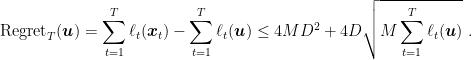
This regret guarantee is very interesting because in the worst case it is still of the order ${O(\sqrt{T})}$ , but in the best case scenario it becomes a constant! In fact, if there exists a ${{\boldsymbol u} \in V}$ such that ${\sum_{t=1}^T \ell_t({\boldsymbol u})=0}$ we get a constant regret. Basically, if the losses are “easy”, the algorithm adapts to this situation and gives us a better regret.

These kind of guarantees are called ${L^\star}$ bounds because they depend on the cumulative competitor loss that can be denoted by ${L^\star}$ .

4. AdaGrad

We now present another application of the regret bound in (2). AdaGrad, that stands for Adaptive Gradient, is an Online Convex Optimization algorithm proposed independentely by (H. B. McMahan and M. J. Streeter, 2010) and (J. Duchi and E. Hazan and Y. Singer, 2010). It aims at being adaptive to the sequence of gradients. It is usually known as a stochastic optimization algorithm, but in reality it was proposed for Online Convex Optimization (OCO). To use it as a stochastic algorithm, you should use an online-to-batch conversion, otherwise you do not have any guarantee of convergence.

We will present a proof that only allows hyperrectangles as feasible sets ${V}$ , on the other hand the restriction makes the proof almost trivial. Let’s see how it works.

AdaGrad has key ingredients:

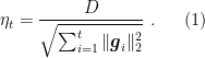
A coordinate-wise learning process;
The adaptive learning rates in (1).

For the first ingredient, as we said, the regret of any OCO problem can be upper bounded by the regret of the Online Linear Optimization (OLO) problem. That is,

$\displaystyle \sum_{t=1}^T \ell_t({\boldsymbol x}_t) - \sum_{t=1}^T \ell_t({\boldsymbol u}) \leq \sum_{t=1}^T \langle {\boldsymbol g}_t, {\boldsymbol x}_t\rangle - \sum_{t=1}^T \langle {\boldsymbol g}_t, {\boldsymbol u}\rangle~.$

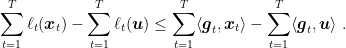
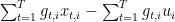
Now, the essential observation is to explicitely write the inner product as a sum of product over the single coordinates:

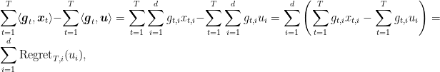
$\displaystyle \sum_{t=1}^T \langle {\boldsymbol g}_t, {\boldsymbol x}_t\rangle - \sum_{t=1}^T \langle {\boldsymbol g}_t, {\boldsymbol u}\rangle = \sum_{t=1}^T \sum_{i=1}^d g_{t,i} x_{t,i} - \sum_{t=1}^T \sum_{i=1}^d g_{t,i} u_i = \sum_{i=1}^d \left(\sum_{t=1}^T g_{t,i} x_{t,i} - \sum_{t=1}^T g_{t,i} u_i\right) = \sum_{i=1}^d \text{Regret}_{T,i}(u_i),$

where we denoted by ${\text{Regret}_{T,i}(u_i)}$ the regret of the 1-dimensional OLO problem over coordinate ${i}$ , that is ${\sum_{t=1}^T g_{t,i} x_{t,i} - \sum_{t=1}^T g_{t,i} u_i}$ . In words, we can decompose the original regret as the sum of ${d}$ OLO regret minimization problems and we can try to focus on each one of them separately.

A good candidate for the 1-dimensional problems is OSD with the learning rates in (1). We can specialize the regret in (2) to the 1-dimensional case for linear losses, so we get for each coordinate ${i}$

$\displaystyle \sum_{t=1}^T g_{t,i} x_{t,i} - \sum_{t=1}^T g_{t,i} u_i \leq \sqrt{2} D_i \sqrt{\sum_{t=1}^T g_{t,i}^2}~.$

This choice gives us the AdaGrad algorithm in Algorithm 1.

adagrad

Putting all together, we have immediately the following regret guarantee.

Theorem 8 Let ${V = \{{\boldsymbol x} : a_i \leq x_i\leq b_i\}}$ with diameters along each coordinate equal to ${D_i=b_i-a_i}$ . Let ${\ell_1, \cdots, \ell_T}$ an arbitrary sequence of convex functions ${\ell_t:{\mathbb R}^d \rightarrow (-\infty, +\infty]}$ subdifferentiable in open sets containing ${V}$ for ${t=1, \dots,T}$ . Pick any ${{\boldsymbol x}_1 \in V}$ and ${\eta_{t,i}=\frac{\sqrt{2}D_i}{2\sqrt{\sum_{j=1}^t g_{j,i}^2}}, \ t=1, \dots, T}$ . Then, ${\forall {\boldsymbol u} \in V}$ , the following regret bound holds

$\displaystyle \text{Regret}_T({\boldsymbol u}) =\sum_{t=1}^T \ell_t({\boldsymbol x}_t) - \sum_{t=1}^T \ell_t({\boldsymbol u}) \leq \sqrt{2} \sum_{i=1}^d D_i \sqrt{\sum_{t=1}^T g_{t,i}^2}~.$

Is this a better regret bound compared to the one in Theorem 2? It depends! To compare the two we have to consider that ${V}$ is a hyperrectangle because the analysis of AdaGrad above only works for hyperrectangle. Then, we have to compare

$\displaystyle \begin{aligned} D\sqrt{\sum_{t=1}^T \|{\boldsymbol g}_{t}\|_2^2} && \text{versus} && \sum_{i=1}^d D_i \sqrt{\sum_{t=1}^T g_{t,i}^2}~. \end{aligned}$

From Cauchy-Schwarz, we have that ${\sum_{i=1}^d D_i \sqrt{\sum_{t=1}^T g_{t,i}^2}\leq D\sqrt{\sum_{t=1}^T \|{\boldsymbol g}_{t}\|_2^2}}$ . So, assuming the same sequence of subgradients, AdaGrad has always a better regret on hyperrectangles. Also, note that

$\displaystyle \sqrt{\sum_{t=1}^T \|{\boldsymbol g}_{t}\|_2^2} \leq \sum_{i=1}^d \sqrt{\sum_{t=1}^T g_{t,i}^2} \leq \sqrt{d} \sqrt{\sum_{t=1}^T \|{\boldsymbol g}_{t}\|_2^2}$

So, in the case that ${V}$ is a hypercube we have ${D_i=D_\infty = \max_{{\boldsymbol x}, {\boldsymbol y}} \|{\boldsymbol x}-{\boldsymbol y}\|_\infty}$ and ${D=\sqrt{d} D_\infty}$ , the bound of AdaGrad is between ${1/\sqrt{d}}$ and ${1}$ times the bound of Theorem 2. In other words, if we are lucky with the subgradients, the particular shape of the domain might save us a factor of ${\sqrt{d}}$ in the guarantee.

Note that the more general analysis of AdaGrad allows to consider arbitrary domains, but it does not change the general message that the best domains for AdaGrad are hypercubes. We will explore this issue of choosing the online algorithm based on the shape of the feasible set ${V}$ when we will introduce Online Mirror Descent.

Hidden in the guarantee is that the biggest advantage of AdaGrad is the property of being coordinate-wise scale-free. That is, if each coordinate of the gradients are multiplied by different constants, the learning rate will automatically scale them back. This is hidden by the fact that the optimal solution ${{\boldsymbol u}}$ would also scale accordingly, but the fixed diameters of the feasible set hide it. This might be useful in the case the ranges of coordinates of the gradients are vastly different one from the other. Indeed, this does happen in the stochastic optimization of deep neural networks, where the first layers have smaller magnitude of the gradients compared to the last layers.

5. History Bits

The adaptive learning rate in (1) first appeared in (M. Streeter and H. B. McMahan, 2010). However, similar methods were used long time before. Indeed, the key observation to approximate oracle quantities with estimates up to time ${t}$ was first proposed in the self-confident algorithms (P. Auer and N. Cesa-Bianchi and C. Gentile, 2002), where the learning rate is inversely proportional to the square root of the cumulative loss of the algorithm, and for smooth losses it implies the ${L^\star}$ bounds similar to the one in Theorem 7.

AdaGrad was proposed in basically identically form independently by two groups at the same conference: (H. B. McMahan and M. J. Streeter, 2010) and (J. Duchi and E. Hazan and Y. Singer, 2010). The analysis presented here is the one in (M. Streeter and H. B. McMahan, 2010) that does not handle generic feasible sets and does not support “full-matrices”, i.e. full-matrix learning rates instead of diagonal ones. However, in machine learning applications AdaGrad is rarely used with a projection step (even if doing so provably destroys the worst-case performance (F. Orabona and D. Pál, 2018)). Also, in the adversarial setting full-matrices do not seem to offer advantages in terms of regret compared to diagonal ones.

Note that the AdaGrad learning rate is usually written as

$\displaystyle \eta_{t,i}=\frac{D_i}{\epsilon+\sqrt{\sum_{j=1}^t g_{j,i}^2}},$

where ${\epsilon>0}$ is a small constant used to prevent division by zero. In reality, ${\epsilon}$ is not necessary and removing it makes the updates scale-free, as stressed in (F. Orabona and D. Pál, 2018).

AdaGrad inspired an incredible number of clones, most of them with similar, worse, or no regret guarantees. The keyword “adaptive” itself has shifted its meaning over time. It used to denote the ability of the algorithm to obtain the same guarantee as it knew in advance a particular property of the data (i.e. adaptive to the gradients/noise/scale = (almost) same performance as it knew the gradients/noise/scale in advance). Indeed, in Statistics this keyword is used with the same meaning. However, “adaptive” has changed its meaning over time. Nowadays, it seems to denote any kind of coordinate-wise learning rates that does not guarantee anything in particular.

6. Exercises

Exercise 1 Prove that the dual norm of ${\|\cdot\|_p}$ is ${\|\cdot\|_q}$ , where ${\frac1p+\frac1q=1}$ and ${p,q\geq1}$ .

Exercise 2 Show that using online subgradient descent on a bounded domain with the learning rates ${\eta_t=O(1/t)}$ with Lipschitz, smooth, and strongly convex functions you can get ${O(\ln(1+L^\star))}$ bounds.

Exercise 3 Prove that the logistic loss ${\ell({\boldsymbol x})=\log(1+\exp(-y\langle{\boldsymbol z},{\boldsymbol x}\rangle))}$ , where ${\|{\boldsymbol z}\|_2\leq 1}$ and ${y \in \{-1,1\}}$ is ${\frac{1}{4}}$ -smooth w.r.t. ${\|\cdot\|_2}$ .

7 Comments

Pingback: Lower Bounds for Online Linear Optimization – Parameter-free Learning and Optimization Algorithms
Pingback: Subgradient Descent Does Not Descend – Parameter-free Learning and Optimization Algorithms
Pingback: Online Mirror Descent II: Regret and Mirror Version – Parameter-free Learning and Optimization Algorithms
Pingback: Online Mirror Descent III: Examples and Learning with Expert Advice – Parameter-free Learning and Optimization Algorithms
Nicolò says:

October 17, 2019 at 4:55 AM

Hi, nice post!
A few comments:
In theorem 8 I think there’s a typo in the definition of $\eta_{t, i}$: in the denominator the sum should be $\sum_{j=1}^t g_{j, i}^2$ as in Algorithm 1, right?
Also, I’m not totally clear about the comparison between Adagrad and OSD. When you say “It is immediate to see..”, why the first term is smaller or equal than the third term?
Based on my reasoning, if we apply Cauchy-Schwartz we get

$$ \sum_{i=1}^d \sqrt{ \sum_{t=1}^T g_{t, i}^2} \leq \sqrt{d} \sqrt{ \sum_{t=1}^T \| g_t \|_2^2 } $$

and then we can multiply both terms by $ D_\infty $. This would be fine if $ D = \sqrt{d} D_\infty $, but that should hold with inequality, i.e. $ D \leq \sqrt{d} D_\infty $. Indeed, assuming we use the definition of D given in lecture 2, $ D = \max_{x, y \in V} \| x – y \| = \| b – a \| = \sqrt{ \sum_{i=1}^d D_i^2} \leq D_\infty \sqrt{d} $. What am I missing?

LikeLike

1. bremen79 says:
  
  October 17, 2019 at 10:19 AM
  
  Thanks for the finding the typo, I fixed it.
  Also, there was some confusion in the text regarding hyperrectangles and hypercubes. I fixed it and made the comparison clearer: It is always better on hyperrectangles and on hypercubes you can might save a factor sqrt{d}. I hope it is better/correct now.
  
  LikeLike
  
Pingback: AdaHedge – Parameter-free Learning and Optimization Algorithms
Anirudh V says:

May 29, 2020 at 10:46 AM

Any hint on how to solve Exercise 2? I followed a similar derivation used for the L* bounds in the notes, but cannot see how we can use the strong convexity to achieve a logarithmic bound

LikeLike

bremen79 says:

May 29, 2020 at 12:53 PM

Hi Anirudh, first let me say that the learning rate in (1) won’t work as it is. You need a hybrid learning rate between the one for strongly convex functions and the one in (1). Start from the one for strongly convex functions and try to make it data-dependent.

LikeLike

1. Anirudh V says:
  
  May 29, 2020 at 9:45 PM
  
  Thanks for the reply! Will try it as you suggested
  
  LikeLike
  
  1. bremen79 says:
    
    March 20, 2021 at 6:38 PM
    
    It seems there was an error in the text of exercise 2, sorry! I have now fixed it…
    
    LikeLike
Pingback: Last Iterate of SGD Converges (Even in Unbounded Domains) – Parameter-free Learning and Optimization Algorithms
Pingback: Almost Sure Convergence of SGD on Smooth Non-Convex Functions – Parameter-free Learning and Optimization Algorithms
Pingback: Neural Network (Maybe) Evolved to Make Adam The Best Optimizer – Parameter-free Learning and Optimization Algorithms
Ella B says:

December 25, 2022 at 9:10 PM

Thankss great blog post

LikeLiked by 1 person