Lower Bounds for Online Linear Optimization

This post is part of the lecture notes of my class “Introduction to Online Learning” at Boston University, Fall 2019. I will publish two lectures per week.

You can find the lectures I published till now here.

In this lecture we will present some lower bounds for online linear optimization (OLO). Remembering that linear losses are convex, this immediately gives us lower bounds for online convex optimization (OCO). We will consider both the constrained and the unconstrained case. The lower bounds are important because they inform us on what are the optimal algorithms and where are the gaps in our knowledge.

1. Lower bounds for Bounded OLO

We will first consider the bounded constrained case. Finding a lower bound accounts to find a strategy for the adversary that forces a certain regret onto the algorithm, no matter what the algorithm does. We will use the probabilistic method to construct our lower bound.

The basic method relies on the fact that for any random variable ${{\boldsymbol z}}$ with domain ${V}$ , and any function ${f}$

$\displaystyle \sup_{{\boldsymbol x} \in V} \ f({\boldsymbol x}) \geq \mathop{\mathbb E} [f({\boldsymbol z})]~.$

For us, it means that we can lower bound the effect of the worst-case sequence of functions with an expectation over any distribution over the functions. If the distribution is chosen wisely, we can expect that gap in the inequality to be small. Why do you rely on expectations rather than actually constructing an adversarial sequence? Because the use of a stochastic loss functions makes very easy to deal with arbitrary algorithms. In particular, we will choose stochastic loss functions that makes the expected loss of the algorithm 0, independently from the strategy of the algorithm.

Theorem 1 Let ${V \subset {\mathbb R}^d}$ be any non-empty bounded closed convex subset. Let ${D = \sup_{{\boldsymbol v},{\boldsymbol w} \in V} \|{\boldsymbol v} - {\boldsymbol w}\|_2}$ be the diameter of ${V}$ . Let ${\mathcal{A}}$ be any (possibly randomized) algorithm for OLO on ${V}$ . Let ${T}$ be any non-negative integer. There exists a sequence of vectors ${{\boldsymbol g}_1, \dots, {\boldsymbol g}_T}$ with ${\|{\boldsymbol g}_t\|_2\leq L}$ and ${{\boldsymbol u} \in V}$ such that the regret of algorithm ${\mathcal{A}}$ satisfies

$\displaystyle \text{Regret}_T({\boldsymbol u}) = \sum_{t=1}^T \langle {\boldsymbol g}_t, {\boldsymbol x}_t \rangle - \sum_{t=1}^T \langle {\boldsymbol g}_t, {\boldsymbol u} \rangle \geq \frac{\sqrt{2} LD \sqrt{T}}{4}~.$

Proof: Let’s denote by ${\text{Regret}_T = \max_{{\boldsymbol u} \in V} \text{Regret}_T({\boldsymbol u})}$ . Let ${{\boldsymbol v}, {\boldsymbol w} \in V}$ such that ${\|{\boldsymbol v}-{\boldsymbol w}\|_2=D}$ . Let ${{\boldsymbol z}=\frac{{\boldsymbol v}-{\boldsymbol w}}{\|{\boldsymbol v}-{\boldsymbol w}\|_2}}$ , so that ${\langle {\boldsymbol z}, {\boldsymbol v}-{\boldsymbol w}\rangle = D}$ . Let ${\epsilon_1, \dots, \epsilon_T}$ be i.i.d. Rademacher random variables, that is ${\Pr[\epsilon_t=1]=\Pr[\epsilon_t=-1]=1/2}$ and set the losses ${{\boldsymbol g}_t=L \epsilon_t {\boldsymbol z}}$ .

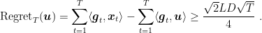
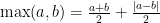
$\displaystyle \begin{aligned} \sup_{{\boldsymbol g}_1, \dots, {\boldsymbol g}_T} \text{Regret}_T &\geq \mathop{\mathbb E}\left[ \sum_{t=1}^T L \epsilon_t \langle {\boldsymbol z}, {\boldsymbol x}_t\rangle - \min_{{\boldsymbol u} \in V} \sum_{t=1}^T L \epsilon_t \langle {\boldsymbol z}, {\boldsymbol u}\rangle\right] = \mathop{\mathbb E}\left[- \min_{{\boldsymbol u} \in V} \sum_{t=1}^T L \epsilon_t \langle {\boldsymbol z}, {\boldsymbol u}\rangle\right] \\ &= \mathop{\mathbb E}\left[\max_{{\boldsymbol u} \in V} \sum_{t=1}^T - L \epsilon_t \langle {\boldsymbol z}, {\boldsymbol u}\rangle\right] = \mathop{\mathbb E}\left[\max_{{\boldsymbol u} \in V} \sum_{t=1}^T L \epsilon_t \langle {\boldsymbol z}, {\boldsymbol u}\rangle\right] \\ &= \mathop{\mathbb E}\left[\max_{{\boldsymbol u} \in \{{\boldsymbol v}, {\boldsymbol w}\}} \sum_{t=1}^T L \epsilon_t \langle {\boldsymbol z}, {\boldsymbol u}\rangle\right] = \mathop{\mathbb E}\left[\frac{1}{2}\sum_{t=1}^T L \epsilon_t \langle {\boldsymbol z}, {\boldsymbol v}+{\boldsymbol w}\rangle + \frac{1}{2}\left| \sum_{t=1}^T L \epsilon_t \langle {\boldsymbol z}, {\boldsymbol v}-{\boldsymbol w}\rangle\right|\right] \\ &= \frac{L}{2}\mathop{\mathbb E}\left[\left|\sum_{t=1}^T \epsilon_t \langle {\boldsymbol z}, {\boldsymbol v}-{\boldsymbol w}\rangle\right|\right] = \frac{LD}{2}\mathop{\mathbb E}\left[\left|\sum_{t=1}^T \epsilon_t \right|\right] \geq \frac{\sqrt{2} LD \sqrt{T}}{4}~. \end{aligned}$

where we used ${\mathop{\mathbb E}[\epsilon_t]=0}$ and the ${\epsilon_t}$ are independent in the first equality, ${\max(a,b)=\frac{a+b}{2}+\frac{|a-b|}{2}}$ in the fourth equality, and Khintchine inequality in the last inequality. $\Box$

We see that the lower bound is a constant multiplicative factor from the upper bound we proved for Online Subgradient Descent (OSD) with learning rates ${\eta_t=\frac{D}{L\sqrt{t}}}$ or ${\eta=\frac{D}{L\sqrt{T}}}$ . This means that OSD is asymptotically optimal with both settings of the learning rate.

At this point there is an important consideration to do: How can this be the optimal regret when we managed to proved better regret, for example with adaptive learning rates? The subtlety is that, constraining the adversary to play ${L}$ -Lipschitz losses, the adversary could always force on the algorithm at least the regret in Theorem 1. However, we can design algorithms that take advantage of suboptimal plays of the adversary. Indeed, for example, if the adversary plays in a way that all the subgradients have the same norm equal to ${L}$ , there is nothing to adapt to!

We now move to the unconstrained case, however first we have to enrich our math toolbox with another essential tool, Fenchel conjugates.

2. Convex Analysis Bits: Fenchel Conjugate

Definition 2 A function ${f:V \subseteq {\mathbb R}^d \rightarrow [-\infty, +\infty]}$ is closed iff ${\{{\boldsymbol x}: f({\boldsymbol x}) \leq \alpha\}}$ is closed for every ${\alpha \in {\mathbb R}}$ .

Note that in a Hausdorff space a function is closed iff it is lower semicontinuos (Bauschke, H. H. and Combettes, P. L., 2011, Lemma 1.24).

Example 1 The indicator function of a set ${V \subset {\mathbb R}^d}$ , is closed iff ${V}$ is closed.

Definition 3 For a function ${f: {\mathbb R}^d\rightarrow [-\infty,\infty]}$ , we define the Fenchel conjugate ${f^\star:{\mathbb R}^d \rightarrow [-\infty,\infty]}$ as

$\displaystyle f^\star({\boldsymbol \theta}) = \sup_{{\boldsymbol x} \in {\mathbb R}^d} \ \langle {\boldsymbol \theta}, {\boldsymbol x}\rangle - f({\boldsymbol x})~.$

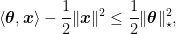
From the definition we immediately obtain the Fenchel’s inequality

$\displaystyle \langle {\boldsymbol \theta}, {\boldsymbol x} \rangle \leq f({\boldsymbol x})+f^\star({\boldsymbol \theta}), \ \forall {\boldsymbol x}, {\boldsymbol \theta} \in {\mathbb R}^d~.$

We have the following useful property for the Fenchel conjugate

Theorem 4 (Rockafellar, R. T., 1970, Corollary 23.5.1 and Theorem 23.5) Let ${f:{\mathbb R}^d \rightarrow (-\infty,+\infty]}$ be convex, proper, and closed. Then

${{\boldsymbol x} \in \partial f^\star({\boldsymbol \theta})}$ iff ${{\boldsymbol \theta} \in \partial f({\boldsymbol x})}$ .

${\langle {\boldsymbol \theta}, {\boldsymbol x}\rangle - f({\boldsymbol x})}$ achieves its supremum in ${{\boldsymbol x}}$ at ${{\boldsymbol x}={\boldsymbol x}^\star}$ iff ${{\boldsymbol x}^\star \in \partial f^\star({\boldsymbol \theta})}$ .

Example 2 Let ${f(x)=\exp(x)}$ , hence we have ${f^\star(\theta)=\max_x \ x\theta - \exp(x)}$ . Solving the optimization, we have that ${x^\star=\ln(\theta)}$ if ${\theta>0}$ and ${f^\star(\theta)=\theta \ln \theta - \theta}$ , ${f^\star(0)=0}$ , and ${f^\star(\theta) = +\infty}$ for ${\theta<0}$ .

Example 3 Consider the function ${f({\boldsymbol x}) = \frac{1}{2}\|{\boldsymbol x}\|^2}$ , where ${\|\cdot\|}$ is a norm in ${{\mathbb R}^d}$ , with dual norm ${\|\cdot\|_\star}$ . We can show that its conjugate is ${f^\star({\boldsymbol \theta})=\frac{1}{2}\|{\boldsymbol \theta}\|^2_\star}$ . From

$\displaystyle \langle {\boldsymbol \theta} , {\boldsymbol x} \rangle - \frac{1}{2}\|{\boldsymbol x}\|^2 \leq \| {\boldsymbol \theta}\|_\star \|{\boldsymbol x}\| - \frac{1}{2}\|{\boldsymbol x}\|^2$

for all ${{\boldsymbol x}}$ . The right hand side is a quadratic function of ${\|{\boldsymbol x}\|}$ , which has maximum value ${\frac{1}{2}\|{\boldsymbol \theta}\|_\star^2}$ . Therefore for all ${{\boldsymbol x}}$ , we have

$\displaystyle \langle {\boldsymbol \theta} , {\boldsymbol x} \rangle - \frac{1}{2}\|{\boldsymbol x}\|^2 \leq \frac{1}{2}\|{\boldsymbol \theta}\|_\star^2,$

which shows that ${f^\star({\boldsymbol \theta}) \leq \frac{1}{2}\|{\boldsymbol \theta}\|^2_\star}$ . To show the other inequality, let ${{\boldsymbol x}}$ be any vector with ${\langle {\boldsymbol \theta}, {\boldsymbol x} \rangle = \|{\boldsymbol \theta}\|_\star \|{\boldsymbol x}\|}$ , scaled so that ${\|{\boldsymbol x}\| = \|{\boldsymbol \theta}\|_\star}$ . Then we have, for this ${{\boldsymbol x}}$ ,

$\displaystyle \langle {\boldsymbol \theta} , {\boldsymbol x} \rangle - \frac{1}{2}\|{\boldsymbol x}\|^2 = \frac{1}{2}\|{\boldsymbol \theta}\|_\star^2,$

which shows that ${f^\star({\boldsymbol \theta}) \geq \frac{1}{2}\|{\boldsymbol \theta}\|^2_\star}$ .

Lemma 5 Let ${f}$ be a function and let ${f^\star}$ be its Fenchel conjugate. For ${a > 0}$ and ${b \in {\mathbb R}}$ , the Fenchel conjugate of ${g({\boldsymbol x}) = a f({\boldsymbol x}) + b}$ is ${g^\star({\boldsymbol \theta}) = a f^\star({\boldsymbol \theta}/a) - b}$ .

Proof: From the definition of conjugate function, we have

$\displaystyle g^\star({\boldsymbol \theta}) = \sup_{{\boldsymbol x} \in {\mathbb R}^d} \langle {\boldsymbol \theta}, {\boldsymbol x}\rangle - a f(x) - b = -b + a \sup_{{\boldsymbol x} \in {\mathbb R}^d} \left\langle \frac{{\boldsymbol \theta}}{a}, {\boldsymbol x}\right\rangle - f(x) = -b + a f^\star\left(\frac{{\boldsymbol \theta}}{a}\right)~.$

$\Box$

Lemma 6 (Bauschke, H. H. and Combettes, P. L., 2011, Example 13.7) Let ${f:{\mathbb R} \rightarrow (-\infty, +\infty]}$ even. Then ${(f \circ \|\cdot\|_2)^\star= f^\star \circ \|\cdot\|_2}$ .

3. Unconstrained OLO

The above lower bound applies only to the constrained setting. In the unconstrained setting, we proved that OSD with ${{\boldsymbol x}_1=\boldsymbol{0}}$ and constant learning rate of ${\eta=\frac{1}{L\sqrt{T}}}$ gives a regret of ${\frac12 L(\|{\boldsymbol u}\|_2^2+1)\sqrt{T}}$ for any ${{\boldsymbol u} \in {\mathbb R}^d}$ . Is this regret optimal? It is clear that the regret must be at least linear in ${\|{\boldsymbol u}\|_2}$ , but is linear enough?

The approach I will follow is to reduce the OLO game to the online game of betting on a coin, where the lower bounds are known. So, let’s introduce the coin-betting online game:

Start with an initial amount of money ${\epsilon>0}$ .
In each round, the algorithm bets a fraction of its current wealth on the outcome of a coin.
The outcome of the coin is revealed and the algorithm wins or lose its bet, 1 to 1.

The aim of this online game is to win as much money as possible. Also, as in all the online games we consider, we do not assume anything on how the outcomes of the coin are decided. Note that this game can also be written as OCO using the log loss.

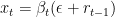
We will denote by ${c_t \in \{-1,1\}, t=1, \dots, T}$ the outcomes of the coin. We will use the absolute value of ${\beta_t \in [-1,1]}$ to denote the fraction of money to bet and its sign to denote on which side we are betting. The money the algorithm has won from the beginning of the game till the end of round ${t}$ will be denoted by ${r_{t}}$ and given that the money are won or lost 1 to 1, we have

$\displaystyle \overbrace{r_t +\epsilon}^{\text{Money at the end of round } t} = \overbrace{r_{t-1} +\epsilon}^{\text{Money at the beginning of round } t} + \overbrace{c_t \beta_t (r_{t-1}+\epsilon)}^\text{Money won or lost} = \epsilon \prod_{i=1}^t (1+\beta_i c_i),$

where we used the fact that ${r_0=0}$ . We will also denote by ${x_t=\beta_t (\epsilon + r_{t-1})}$ the bet of the algorithm on round ${t}$ .

If we got all the outcomes of the coin correct, we would double our money in each round, so that ${\epsilon+r_T=\epsilon 2^T}$ . However, given the adversarial nature of the game, we can actually prove a stronger lower bound to the maximum wealth we can gain.

Theorem 7 (Cesa-Bianchi, N. and Lugosi, G. , 2006, a simplified statement of Theorem 9.2) Let ${T\geq 21}$ . Then, for any betting strategy with initial money ${\epsilon>0}$ that bets fractions of its current wealth, there exists a sequence of coin outcomes ${c_t}$ , such that

$\displaystyle \epsilon + \sum_{t=1}^T c_t x_t \leq \frac{1}{\sqrt{T}}\max_{ -1\leq\beta\leq 1 } \ \epsilon \prod_{t=1}^T (1+\beta c_t) \leq \frac{\epsilon}{\sqrt{T}} \exp\left(\frac{\ln 2(\sum_{t=1}^T c_t)^2}{T}\right) ~.$

Now, let’s connect the coin-betting game with OLO. Remember that proving a regret guarantee in OLO consists in showing

$\displaystyle \sum_{t=1}^T \langle {\boldsymbol g}_t, {\boldsymbol x}_t\rangle - \sum_{t=1}^T \langle {\boldsymbol g}_t,{\boldsymbol u}\rangle \leq \psi_T({\boldsymbol u}), \ \forall {\boldsymbol u} \in {\mathbb R}^d,$

for some function ${\psi_T}$ , where we want the dependency on ${T}$ to be sublinear. Using our new learned concept of Fenchel conjugate, this is equivalent to prove that

$\displaystyle \begin{aligned} \sum_{t=1}^T \langle {\boldsymbol g}_t, {\boldsymbol x}_t\rangle \leq \inf_{{\boldsymbol u}} \ \sum_{t=1}^T \langle {\boldsymbol g}_t,{\boldsymbol u}\rangle + \psi_T({\boldsymbol u}) = - \sup_{{\boldsymbol u}} \ -\left\langle \sum_{t=1}^T {\boldsymbol g}_t,{\boldsymbol u}\right\rangle - \psi_T({\boldsymbol u}) = - \psi_T^\star\left(-\sum_{t=1}^T {\boldsymbol g}_t\right)~. \end{aligned}$

Hence, for a given online algorithm we can prove regret bounds proving that there exists a function ${\psi_T}$ or equivalently finding its conjugate ${\psi^\star_T}$ . Similarly, proving a lower bound in unconstrained OLO means finding a sequence of ${{\boldsymbol g}_t}$ and a function ${\psi_T}$ or a function ${\psi^\star_T}$ that lower bound the regret or the cumulative losses of the algorithm respectively.

Without any other information, it can be challenging to guess what is the slowest increasing function ${\psi_T}$ . So, we restrict our attention to online algorithms that guarantee a constant regret against the zero vector. This immediately imply the following important consequence.

Theorem 8 Let ${\epsilon(t)}$ a non-decreasing function of the index of the rounds and ${\mathcal{A}}$ an OLO algorithm that guarantees ${\text{Regret}_t(\boldsymbol{0})\leq \epsilon(t)}$ for any sequence of ${{\boldsymbol g}_1,\dots,{\boldsymbol g}_t \in {\mathbb R}^d}$ with ${\|{\boldsymbol g}_i\|_2\leq 1}$ . Then, there exists ${\beta_t}$ such that ${{\boldsymbol x}_t= {\boldsymbol \beta}_t (\epsilon(T)-\sum_{i=1}^{t-1} \langle {\boldsymbol g}_i, {\boldsymbol x}_i\rangle)}$ and ${\|\beta_t\|_2\leq1}$ for ${t=1, \dots, T}$ .

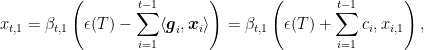
Proof: Define 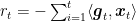${r_t=-\sum_{i=1}^t \langle {\boldsymbol g}_t, {\boldsymbol x}_t\rangle}$ the “reward” of the algorithm. So, we have

$\displaystyle \text{Regret}_T({\boldsymbol u}) =\sum_{t=1}^T \langle {\boldsymbol g}_t, {\boldsymbol x}_t\rangle - \sum_{t=1}^T \langle {\boldsymbol g}_t, {\boldsymbol u}\rangle = -r_T + \left\langle \sum_{t=1}^T g_t, {\boldsymbol u}\right\rangle~.$

Since, we assumed that ${\text{Regret}_t(\boldsymbol{0})\leq \epsilon(t)}$ , we always have ${r_t \geq -\epsilon(t)}$ . Using this, we claim that ${\|{\boldsymbol x}_t\|_2 \leq r_{t-1} + \epsilon(t)}$ for all ${t=1,\dots,T}$ . To see this, assume that there is a sequence ${{\boldsymbol g}_1, \dots, {\boldsymbol g}_{t-1}}$ that gives ${\|{\boldsymbol x}_t\|_2 > r_{t-1} + \epsilon(t)}$ . We then set ${{\boldsymbol g}_t=\frac{{\boldsymbol x}_t}{\|{\boldsymbol x}_t\|_2}}$ . For this sequence, we would have ${r_t = r_{t-1} - \|{\boldsymbol x}_t\|_2 < -\epsilon(t)}$ , that contradicts the observation that ${r_t \geq -\epsilon(t)}$ .

So, from the fact that ${\|{\boldsymbol x}_t\|_2 \leq r_{t-1} + \epsilon(t) \leq r_{t-1} + \epsilon(T)}$ we have that there exists ${\beta_t}$ such that ${{\boldsymbol x}_t = {\boldsymbol \beta}_t (\epsilon(T)+r_{t-1})}$ for a ${{\boldsymbol \beta}_t}$ and ${\|{\boldsymbol \beta}_t\|_2 \leq 1}$ . $\Box$

This theorem informs us of something important: any OLO algorithm that suffer a non-decreasing regret against the null competitor must predict in the form of a “vectorial” coin-betting algorithm. This immediately implies the following.

Theorem 9 Let ${T\geq 21}$ . For any OLO algorithm, under the assumptions of Theorem 8, there exist a sequence of ${{\boldsymbol g}_1,\dots,{\boldsymbol g}_T \in {\mathbb R}^d}$ with ${\|{\boldsymbol g}_t\|_2\leq 1}$ and ${{\boldsymbol u}^\star \in {\mathbb R}^d}$ , such that

$\displaystyle \begin{aligned} \sum_{i=1}^t \langle {\boldsymbol g}_t, {\boldsymbol x}_t\rangle -\sum_{t=1}^T \langle {\boldsymbol g}_t, {\boldsymbol u}^\star\rangle \geq 0.8 \|{\boldsymbol u}^\star\|_2 \sqrt{T} \left(\sqrt{0.3 \ln \frac{0.8 \|{\boldsymbol u}^\star\|_2 T }{\epsilon(T)}}-1\right)+\epsilon(T)\left(1-\frac{1}{\sqrt{T}}\right)~. \end{aligned}$

Proof: The proof works by reducing the OLO game to a coin-betting game and then using the upper bound to the reward for coin-betting games.

First, set ${{\boldsymbol g}_t=[-c_t,0,\dots,0]}$ , where ${c_t \in \{-1,1\}}$ will be defined in the following, so that ${\langle {\boldsymbol g}_t, {\boldsymbol x}\rangle= -c_t x_1}$ for any ${{\boldsymbol x} \in {\mathbb R}^d}$ . Given Theorem 8, we have that the first coordinate of ${{\boldsymbol x}_t}$ has to satisfy

$\displaystyle x_{t,1} = \beta_{t,1} \left(\epsilon(T) - \sum_{i=1}^{t-1} \langle {\boldsymbol g}_i, {\boldsymbol x}_i\rangle\right) = \beta_{t,1} \left(\epsilon(T) + \sum_{i=1}^{t-1} c_i, x_{i,1}\right),$

for some ${\beta_{t,1}}$ such that ${|\beta_{t,1}|\leq 1}$ . Hence, the above is nothing else than a coin-betting algorithm that bets ${x_{t,1}}$ money on the outcome of a coin ${c_t}$ , with initial money ${\epsilon(T)}$ . This means that the upper bound to its reward in Theorem 7 applies: there exists a sequence of ${c_t}$ such that

$\displaystyle \sum_{t=1}^T \langle {\boldsymbol g}_t, {\boldsymbol x}_t\rangle - \epsilon(T) = -\sum_{t=1}^T c_t x_{t,1} - \epsilon(T) \geq -\frac{\epsilon(T)}{\sqrt{T}} \exp\left(\frac{\ln 2(\sum_{t=1}^T c_t)^2}{T}\right) = -\sum_{t=1}^T c_t u^\star_{1} + f^\star(|u^\star_1|) = \sum_{t=1}^T \langle {\boldsymbol g}_t, {\boldsymbol u}\rangle + f^\star(\|{\boldsymbol u}^\star\|_2),$

where ${g^\star}$ is the Fenchel conjugate of the function ${f(x)=\frac{\epsilon(T)}{\sqrt{T}} \exp\left(\frac{x^2 \ln 2}{T}\right)}$ and ${u^\star = f'(\sum_{t=1}^T c_t) \in R}$ by Theorem 4 part 2. Using the closed form solution for the Fenchel conjugate as well as its lower bound from (Orabona, F. and Pal, D., 2016) and reordering the terms, we get the stated bound. $\Box$

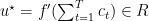
From the above theorem we have that OSD with learning rate ${\eta=\frac{\alpha}{L \sqrt{T}}}$ does not have the optimal dependency on ${\|{\boldsymbol u}\|_2}$ for any ${\alpha>0}$ .

In the future classes, we will see that the connection between coin-betting and OLO can also be used to design OLO algorithm. This will give us optimal unconstrained OLO algorithms with the surprising property of not requiring a learning rate at all.

4. History Bits

The lower bound for OCO is quite standard, the proof presented is a simplified version of the one in (F. Orabona and D. Pál, 2018).

On the other hand, both the online learning literature and the optimization one almost ignored the issue of lower bounds for the unconstrained case. The connection between coin betting and OLO was first unveiled in (Orabona, F. and Pal, D., 2016). Theorem 8 is an unpublished result by Ashok Cutkosky (Thanks for allowing me to use it here!), that proved similar and more general results in his PhD thesis (Cutkosky, A., 2018). Theorem 9 is new, by me. (McMahan, B. and Abernethy, J., 2013) implicitly also proposed using the conjugate function for lower bound in unconstrained OLO.

There is a caveat in the unconstrained lower bound: A stronger statement would be to choose the norm of ${{\boldsymbol u}^\star}$ beforehand. To do this, we would have to explicitely construct the sequence of the ${c_t}$ . One way to do is to use Rademacher coins and then leverage again the hypothesis on the regret against the null competitor. This route was used in (M. Streeter and B. McMahan, 2012), but the proof relied on assuming the value of the global optimum of a non-convex function with an infinite number of local minima. The correct proof avoiding that step was then given in (Orabona, F., 2013). Yet, the proof presented here, that converts reward upper bounds in regret lower bound, is simpler in spirit and (I hope!) more understandable. Given that, as far as I know, this is the first time that unconstrained OLO lower bounds are taught in a class, I valued simplicity over generality.

5. Exercises

Exercise 1 Fix ${U>0}$ . Mimicking the proof of Theorem 1, prove that for any OCO algorithm there exists a ${{\boldsymbol u}^\star}$ and a sequence of loss functions such that ${\text{Regret}_T({\boldsymbol u}^\star)\geq\frac{\sqrt{2}}{2}\|{\boldsymbol u}^\star\|_2 L \sqrt{T}}$ where ${\|{\boldsymbol u}^\star\|_2=U}$ and the loss functions are ${L}$ -Lipschitz w.r.t. ${\|\cdot\|_2}$ .

Exercise 2 Extend the proof of Theorem 1 to an arbitrary norm ${\|\cdot\|}$ to measure the diameter of ${V}$ and with ${\|{\boldsymbol g}_t\|_\star \leq L}$ .

Exercise 3 Let ${f : {\mathbb R}^d \rightarrow (-\infty, +\infty]}$ be even. Prove that ${f^\star}$ is even

Exercise 4 Find the exact expression of the conjugate function of ${f(x)=\alpha \exp(\beta x^2)}$ , for ${\alpha, \beta>0}$ . Hint: Wolfram Alpha or any other kind of symbolic solver can be very useful for this type of problems.

3 Comments

bremen79 says:

September 25, 2019 at 12:31 PM

Update: Fixed a problem in the proof of Theorem 8 that one of my students anonymously posted on our internal forum.

LikeLike

Pingback: Follow-The-Regularized-Leader I: Regret Equality – Parameter-free Learning and Optimization Algorithms
Mass says:

January 20, 2020 at 11:41 AM

Hi Francesco,

First fo all, nice post! I’m pretty sure I may be missing something simple, but I don’t quite see why Theorem 1 requires a constrained domain. If we remove that assumption, where does the proof break? We could define v and w in a slightly different way. Define them such that ||v-w||=1, and change the equality at the beginning of line 3 of the proof to an inequality (restricting the optimization domain to {v, w}). Then, I feel that all of the steps would still be valid. Of course, the diameter D won’t show up anymore, but that’s a constant. What’s wrong with these modifications?

Thanks!

LikeLike

1. bremen79 says:
  
  January 20, 2020 at 4:09 PM
  
  Hi Mass,
  
  yes, you are very right! The theorem would work also for unbounded domains. However, the resulting lower bound would be supoptimal because it would lack of the logarithmic factor we get from the other proof. I guess I should change a bit the text to explain this bit.
  
  LikeLike

Share this:

Like this:

Related

Leave a Reply Cancel reply