AdaHedge

Disclaimer: This post assumes that you understand how FTRL works. If not, please take a look here.

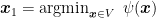
In this post, I explain a variation of the EG/Hedge algorithm, called AdaHedge. The basic idea is to design an algorithm that is adaptive to the sum of the squared ${L_\infty}$ norm of the losses, without any prior information on the range of the losses.

First, consider the case in which we use as constant regularizer the negative entropy 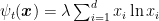${\psi_t({\boldsymbol x}) = \lambda \sum_{i=1}^d x_i \ln x_i}$ , where ${\lambda>0}$ will be determined in the following and ${V}$ is the simplex in ${{\mathbb R}^d}$ . Using FTRL with linear losses with this regularizer, we immediately obtain

$\displaystyle \begin{aligned} \text{Regret}_T({\boldsymbol u}) &\leq \lambda \left(\ln d + \sum_{i=1}^d u_i \ln u_i\right) + \sum_{t=1}^T \left(F_t({\boldsymbol x}_t) - F_{t+1}({\boldsymbol x}_{t+1}) + \langle {\boldsymbol g}_t, {\boldsymbol x}_t\rangle\right) \\ &\leq \lambda \ln d + \sum_{t=1}^T \left(F_t({\boldsymbol x}_t) - F_{t+1}({\boldsymbol x}_{t+1}) + \langle {\boldsymbol g}_t, {\boldsymbol x}_t\rangle\right), \end{aligned}$

where we upper bounded the negative entropy of ${{\boldsymbol u}}$ with 0. Using the strong convexity of the regularizer w.r.t. the ${L_1}$ norm and Lemma 4 here, we would further upper bound this as

$\displaystyle \text{Regret}_T({\boldsymbol u}) \leq \lambda \ln d + \sum_{t=1}^T \frac{\|{\boldsymbol g}_t\|^2_\infty}{2\lambda}~.$

This suggests that the optimal ${\lambda}$ should be ${\lambda = \sqrt{\frac{\sum_{t=1}^T \|{\boldsymbol g}_t\|^2_\infty}{2\ln d}}}$ . However, as we have seen for L* bounds, this choice of any parameter of the algorithm is never feasible. Hence, exactly as we did for L* bounds, we might think of using an online version of this choice

$\displaystyle \label{eq:adahedge_simple} \psi_t({\boldsymbol x}) = \lambda_t \sum_{i=1}^d x_i \ln x_i \quad \text{ where } \quad \lambda_t = \frac{1}{\alpha}\sqrt{\sum_{i=1}^{t-1} \|{\boldsymbol g}_i\|^2_\infty}, \ \ \ \ \ (1)$

where ${\alpha>0}$ is a constant that will be determined later. An important property of such choice is that it gives rise to an algorithm that is scale-free, that is its predictions ${{\boldsymbol x}_t}$ are invariant from the scaling of the losses by any constant factor. This is easy to see because

$\displaystyle x_{t,j} \propto \exp\left(- \frac{\alpha \sum_{i=1}^{t-1} g_{i,j}}{\sqrt{\sum_{i=1}^{t-1} \|{\boldsymbol g}_i\|^2_\infty}}\right), \ \forall i=1,\dots, d~.$

Note that this choice makes the regularizer non-decreasing over time and immediately gives us

$\displaystyle \text{Regret}_T({\boldsymbol u}) \leq \lambda_T \ln d + \sum_{t=1}^T \frac{\|{\boldsymbol g}_t\|^2_\infty}{2\lambda_{t}} = \frac{\ln d}{\alpha} \sqrt{\sum_{t=1}^{T} \|{\boldsymbol g}_t\|^2_\infty} + \alpha \sum_{t=1}^T \frac{\|{\boldsymbol g}_t\|^2_\infty}{2 \sqrt{\sum_{i=1}^{t-1} \|{\boldsymbol g}_i\|^2_\infty}}~.$

At this point, we might be tempted to use Lemma 1 from the L* post to upper bound the sum in the upper bound, but unfortunately we cannot! Indeed, the denominator does not contain the term ${\|{\boldsymbol g}_t\|_\infty^2}$ . We might add a constant to ${\lambda_t}$ , but that would destroy the scale-freeness of the algorithm. However, it turns out that we can still prove our bound without any change to the regularizer. The key observation is that we can bound the term ${F_t({\boldsymbol x}_t) - F_{t+1}({\boldsymbol x}_{t+1}) + \langle {\boldsymbol g}_t, {\boldsymbol x}_t\rangle}$ in two different ways. The first way is the one above, while the other one is

$\displaystyle \begin{aligned} F_t({\boldsymbol x}_t) - F_{t+1}({\boldsymbol x}_{t+1}) + \langle {\boldsymbol g}_t, {\boldsymbol x}_t\rangle &\leq F_t({\boldsymbol x}_{t+1}) - F_{t+1}({\boldsymbol x}_{t+1}) + \langle {\boldsymbol g}_t, {\boldsymbol x}_t\rangle\\ &=\psi_t({\boldsymbol x}_{t+1}) + \sum_{i}^{t-1} \langle {\boldsymbol g}_i, {\boldsymbol x}_{t+1}\rangle - \psi_{t+1}({\boldsymbol x}_{t+1}) - \sum_{i=1}^t \langle {\boldsymbol g}_i, {\boldsymbol x}_{t+1}\rangle \\ &\leq -\langle {\boldsymbol g}_t, {\boldsymbol x}_{t+1}\rangle + \langle {\boldsymbol g}_t, {\boldsymbol x}_t\rangle \\ &\leq 2\|{\boldsymbol g}_t\|_\infty, \end{aligned}$

where we used the definition of ${{\boldsymbol x}_{t+1}}$ and the fact that the regularizer is non-decreasing over time. So, we can now write

$\displaystyle \begin{aligned} \sum_{t=1}^T F_t({\boldsymbol x}_t) - F_{t+1}({\boldsymbol x}_{t+1}) + \langle {\boldsymbol g}_t, {\boldsymbol x}_t\rangle &\leq \sum_{t=1}^T \min\left( \frac{\alpha \|{\boldsymbol g}_t\|_\infty^2}{2 \sqrt{\sum_{i=1}^{t-1} \|{\boldsymbol g}_i\|_\infty^2}}, 2\|{\boldsymbol g}_t\|_\infty \right) \\ &= 2 \sum_{t=1}^T \sqrt{\min\left( \frac{\alpha^2 \|{\boldsymbol g}_t\|_\infty^4}{16\sum_{i=1}^{t-1} \|{\boldsymbol g}_i\|_\infty^2}, \|{\boldsymbol g}_t\|^2_\infty \right)} \\ &\leq 2\sum_{t=1}^T \sqrt{\frac{2}{\frac{16\sum_{i=1}^{t-1} \|{\boldsymbol g}_i\|_\infty^2}{\alpha^2 \|{\boldsymbol g}_t\|_\infty^4} + \frac{1}{\|{\boldsymbol g}_t\|^2_\infty}} } \\ &=2 \sum_{t=1}^T \sqrt{2}\frac{\alpha \|{\boldsymbol g}_t\|_\infty^2}{\sqrt{\alpha^2 \|{\boldsymbol g}_t\|^2_\infty+16\sum_{i=1}^{t-1} \|{\boldsymbol g}_i\|_\infty^2}}, \end{aligned}$

where we used the fact that the minimum between two numbers is less than their harmonic mean. Assuming ${\alpha\geq 4}$ and using Lemma 1 here, we have

$\displaystyle \sum_{t=1}^T F_t({\boldsymbol x}_t) - F_{t+1}({\boldsymbol x}_{t+1}) + \langle {\boldsymbol g}_t, {\boldsymbol x}_t\rangle \leq \frac{\sqrt{2}}{2}\sum_{t=1}^T \frac{\alpha \|{\boldsymbol g}_t\|_\infty^2}{\sqrt{\sum_{i=1}^{t} \|{\boldsymbol g}_i\|_\infty^2}} \leq \sqrt{2 \sum_{t=1}^{T} \|{\boldsymbol g}_t\|_\infty^2}$

and

$\displaystyle \label{eq:adahedge1} \text{Regret}_T({\boldsymbol u}) \leq \left(\frac{\ln d}{\alpha} + \alpha \sqrt{2}\right)\sqrt{\sum_{t=1}^{T} \|{\boldsymbol g}_t\|^2_\infty} ~. \ \ \ \ \ (2)$

The bound and the assumption on ${\alpha}$ suggest to set ${\alpha = \max(4, 2^{-1/4} \sqrt{\ln d})}$ . To summarize, we obtained a scale-free algorithm with regret bound ${O(\sqrt{\ln d \sum_{t=1}^T \|{\boldsymbol g}_t\|^2_\infty})}$ .

We might consider ourselves happy, but there is a clear problem in the above algorithm: the choice of ${\lambda_t}$ in the time-varying regularizer strictly depends on our upper bound. So, a loose bound will result in a poor choice of the regularization! In general, every time we use a part of the proof in the design of an algorithm we cannot expect an exciting empirical performance, unless our upper bound was really tight. So, can we design a better regularizer? Well, we need a better upper bound!

Let’s consider a generic regularizer ${\psi_t({\boldsymbol x})=\lambda_t \psi({\boldsymbol x})}$ and its corresponding FTRL with linear losses regret upper bound

$\displaystyle \text{Regret}_T({\boldsymbol u}) \leq \lambda_T (\psi({\boldsymbol u}) -\inf_{{\boldsymbol x} \in V} \psi({\boldsymbol x}))+ \sum_{t=1}^T \left(F_t({\boldsymbol x}_t) - F_{t+1}({\boldsymbol x}_{t+1}) + \langle {\boldsymbol g}_t, {\boldsymbol x}_t\rangle\right),$

where we assume ${\lambda_t}$ to be non-decreasing in time.

Now, observe that the sum is unlikely to disappear for this kind of algorithms, so we could try to make the term ${\lambda_T (\psi({\boldsymbol u}) -\inf_{{\boldsymbol x} \in V} \psi({\boldsymbol x}))}$ of the same order of the sum. So, we would like to set ${\lambda_t}$ of the same order of ${\sum_{i=1}^t\left(F_i({\boldsymbol x}_i) - F_{i+1}({\boldsymbol x}_{i+1}) + \langle {\boldsymbol g}_i, {\boldsymbol x}_i\rangle\right)}$ . However, this approach would cause an annoying recurrence. So, using the fact that ${\lambda_t}$ is non-decreasing, let’s upper bound the terms in the sum just a little bit:

$\displaystyle \begin{aligned} F_t({\boldsymbol x}_t) - F_{t+1}({\boldsymbol x}_{t+1}) + \langle {\boldsymbol g}_t, {\boldsymbol x}_t\rangle &= F_t({\boldsymbol x}_t)- \lambda_{t+1} \psi({\boldsymbol x}_{t+1}) - \sum_{i=1}^t \langle {\boldsymbol g}_i, {\boldsymbol x}_{t+1}\rangle + \langle {\boldsymbol g}_t, {\boldsymbol x}_t\rangle\\ &\leq F_t({\boldsymbol x}_t) - \lambda_{t} \psi({\boldsymbol x}_{t+1}) - \sum_{i=1}^t \langle {\boldsymbol g}_i, {\boldsymbol x}_{t+1}\rangle + \langle {\boldsymbol g}_t, {\boldsymbol x}_t\rangle\\ &\leq F_t({\boldsymbol x}_t) - \min_{{\boldsymbol x} \in V} \left(\lambda_{t} \psi({\boldsymbol x}) + \sum_{i=1}^t \langle {\boldsymbol g}_i, {\boldsymbol x}\rangle\right) + \langle {\boldsymbol g}_t, {\boldsymbol x}_t\rangle :=\delta_t~. \end{aligned}$

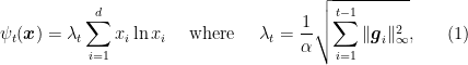
Now, we can set ${\lambda_t = \frac{1}{\alpha^2} \sum_{i=1}^{t-1} \delta_i}$ for ${t\geq 2}$ , ${\lambda_1=0}$ , and ${{\boldsymbol x}_1 = \mathop{\mathrm{argmin}}_{{\boldsymbol x} \in V} \ \psi({\boldsymbol x})}$ . This immediately implies that

$\displaystyle \text{Regret}_T({\boldsymbol u}) \leq \left(\psi({\boldsymbol u}) -\inf_{{\boldsymbol x} \in V} \psi({\boldsymbol x}) + \alpha^2\right)\lambda_{T+1}~.$

Setting ${\psi}$ to be equal to the negative entropy, we get an algorithm known as AdaHedge. It is easy to see that this choice makes the algorithm scale-free as well.

With this choice of the regularizer, we can simplify a bit the expression of ${\delta_t}$ . For ${t=1}$ , we have ${\delta_1=\langle {\boldsymbol g}_1, {\boldsymbol x}_1\rangle - \min_{{\boldsymbol x} \in V} \ \langle{\boldsymbol g}_1, {\boldsymbol x}\rangle}$ . Instead, for ${t\geq2}$ , using the properties of the Fenchel conjugates, we have that

$\displaystyle \delta_t =\lambda_t \ln \frac{\sum_{j=1}^d \exp\left(\theta_{t+1,j}/\lambda_t\right)}{\sum_{j=1}^d \exp\left(\theta_{t,j}/\lambda_t\right)}+\langle {\boldsymbol g}_t,{\boldsymbol x}_t\rangle =\lambda_t \ln \left(\sum_{j=1}^d x_{t,j}\exp\left(-g_{t,j}/\lambda_t\right)\right)+\langle {\boldsymbol g}_t,{\boldsymbol x}_t\rangle~.$

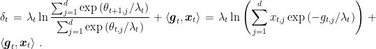
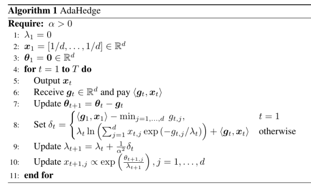
Overall, we get the pseudo-code of AdaHedge in Algorithm 1.

Screenshot_20200503_170947

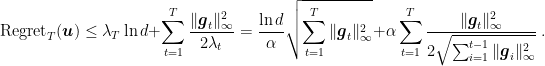
So, now we need an upper bound for ${\lambda_T}$ . Observe that ${\lambda_{t+1}=\lambda_{t} + \frac{1}{\alpha^2} \delta_t}$ . Moreover, as we have done before, we can upper bound ${\delta_t}$ in two different ways. In fact, from Lemma 4 here, we have ${\delta_t \leq \frac{\|{\boldsymbol g}_t\|^2_\infty}{2\lambda_t}}$ for ${t\geq2}$ . Also, denoting by ${\tilde{{\boldsymbol x}}_{t+1} = \mathop{\mathrm{argmin}}_{{\boldsymbol x} \in V} \lambda_{t} \psi({\boldsymbol x}) + \sum_{i=1}^t \langle {\boldsymbol g}_i, {\boldsymbol x}\rangle}$ , we have

$\displaystyle \begin{aligned} \delta_t &= F_t({\boldsymbol x}_t) - \min_{{\boldsymbol x} \in V} \left(\lambda_{t} \psi({\boldsymbol x}) + \sum_{i=1}^t \langle {\boldsymbol g}_i, {\boldsymbol x}\rangle\right) + \langle {\boldsymbol g}_t, {\boldsymbol x}_t\rangle = F_t({\boldsymbol x}_t) - \lambda_{t} \psi(\tilde{{\boldsymbol x}}_{t+1}) - \sum_{i=1}^t \langle {\boldsymbol g}_i, \tilde{{\boldsymbol x}}_{t+1}\rangle + \langle {\boldsymbol g}_t, {\boldsymbol x}_t\rangle \\ &\leq F_t(\tilde{{\boldsymbol x}}_{t+1}) - \lambda_{t} \psi(\tilde{{\boldsymbol x}}_{t+1}) - \sum_{i=1}^t \langle {\boldsymbol g}_i, \tilde{{\boldsymbol x}}_{t+1}\rangle + \langle {\boldsymbol g}_t, {\boldsymbol x}_t\rangle = -\langle {\boldsymbol g}_t, \tilde{{\boldsymbol x}}_{t+1}\rangle + \langle {\boldsymbol g}_t, {\boldsymbol x}_t\rangle \leq 2\|{\boldsymbol g}_t\|_\infty~. \end{aligned}$

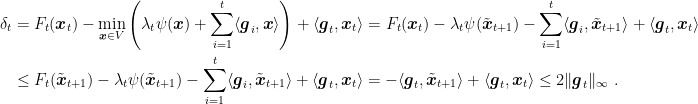
Hence, we have

$\displaystyle \begin{aligned} \lambda_1 &= 0, \\ \lambda_2 &\leq 2 \alpha \|{\boldsymbol g}_1\|_\infty,\\ \lambda_{t+1} &= \lambda_t + \frac{\delta_t}{\alpha^2} \leq \lambda_t + \frac{1}{\alpha^2} \min\left(2\|{\boldsymbol g}_t\|_\infty,\frac{\|{\boldsymbol g}_t\|^2_\infty}{2\lambda_t} \right), \ \forall t\geq 2~. \end{aligned}$

We can solve this recurrence using the following Lemma, where ${\Delta_t=\lambda_t}$ and ${a_t=\|{\boldsymbol g}_t\|_\infty}$ .

Lemma 1. Let ${\{a_t\}_{t=1}^\infty}$ be any sequence of non-negative real numbers. Suppose that ${\{\Delta_t\}_{t=0}^\infty}$ is a sequence of non-negative real numbers satisfying

$\displaystyle \Delta_0 = 0 \qquad \text{and} \qquad \Delta_t \le \Delta_{t-1} + \min \left\{ b a_t, \ c \frac{a_t^2}{2\Delta_{t-1}} \right\} \quad \text{for any } t \ge 1~.$

Then, for any ${T \ge 0}$ , ${\Delta_T \le \sqrt{(b^2 + c)\sum_{t=1}^T a_t^2}}$ .

Proof: Observe that

$\displaystyle \Delta_T^2 = \sum_{t=1}^T (\Delta_t^2 - \Delta_{t-1}^2) = \sum_{t=1}^T \left[(\Delta_t - \Delta_{t-1})^2 + 2 (\Delta_t - \Delta_{t-1}) \Delta_{t-1}\right]~.$

We bound each term in the sum separately. The left term of the minimum inequality in the definition of ${\Delta_t}$ gives ${ (\Delta_t - \Delta_{t-1})^2 \le b^2 a_t^2}$ , while the right term gives ${2 (\Delta_t - \Delta_{t-1}) \Delta_{t-1} \le c a_t^2}$ . So, we conclude ${\Delta_T^2 \leq (b^2+c) \sum_{t=1}^T a_t^2}$ . $\Box$

So, overall we got

$\displaystyle \text{Regret}_T({\boldsymbol u}) \leq \left(\psi({\boldsymbol u}) -\inf_{{\boldsymbol x} \in V} \psi({\boldsymbol x}) + \alpha^2\right)\lambda_{T+1} \leq \left(\frac{\psi({\boldsymbol u}) -\inf_{{\boldsymbol x} \in V} \psi({\boldsymbol x})}{\alpha^2} + 1\right)\sqrt{\left(4+\alpha^2\right) \sum_{t=1}^T \|{\boldsymbol g}_t\|_\infty^2},$

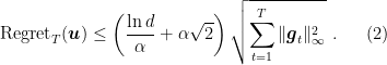
and setting ${\alpha=\sqrt{\ln d}}$ , we have

$\displaystyle \text{Regret}_T({\boldsymbol u}) \leq 2\sqrt{\left(4+\ln d\right) \sum_{t=1}^T \|{\boldsymbol g}_t\|_\infty^2}~.$

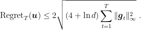
Note that this is roughly the same regret in (2), but the very important difference is that this new regret bound depends on the much tighter quantity ${\lambda_{T+1}}$ , that we upper bounded with ${O(\sqrt{\sum_{t=1}^T \|{\boldsymbol g}_t\|_\infty^2})}$ , but in general will be much smaller than that. For example, ${\lambda_{T+1}}$ can be upper bounded using the tighter local norms, see the analysis of Exp3. Instead, in the first solution, the regret will always be dominated by the term ${\sqrt{\sum_{t=1}^T \|{\boldsymbol g}_t\|_\infty^2}}$ because we explicitly use it in the regularizer!

There is an important lesson to be learned from AdaHedge: the regret is not the full story and algorithms with the same worst-case guarantee can exhibit vastly different empirical behaviors. Unfortunately, this message is rarely heard and there is a part of the community that focuses too much on the worst-case guarantee rather than on the empirical performance. Even worse, sometimes people favor algorithms with a “more elegant analysis” completely ignoring the likely worse empirical performance.

1. History Bits

The use of FTRL with the regularizer in (1) was proposed in (Orabona and Pál, 2015), I presented a simpler version of their proof that does not require Fenchel conjugates. The AdaHedge algorithm was introduced in (van Erven et al., 2011) and refined in (de Rooij et al., 2014). The analysis reported here is from (Orabona and Pál, 2015), that generalized AdaHedge to arbitrary regularizers in AdaFTRL. Additional properties of AdaHedge for the stochastic case were proven in (van Erven et al., 2011).

2. Exercises

Exercise 1. Implement AdaHedge and compare its empirical performance to FTRL with the time-varying regularizer in (1).

2 Comments

mihahauke says:

September 28, 2020 at 5:10 AM

Hi, again your blog is making my life better. I think that it should be ‘\alpha = max (4 …)’ in (2) not min and the inequality in the assumption should \geq not strict. And It’s going to be 4 anyway unless d is in billions. Aaaand if we assume \alpha \leq 4, 4 ends up being optimal so perhaps just set alpha to 4?

Typo in bounding lambda middle step of the third equation (“Hence, we have …” : ‘\lambda_{t+1} = \lambda{t} +\alpha\delta_t’ instead of ‘\lambda_{t+1} = \lambda{t} +\farc{\delta_t}{\alpha^2}’
Missing brackets in the first sum of proof of lemma 1 (for clarity).

LikeLike

1. bremen79 says:
  
  September 28, 2020 at 9:54 AM
  
  Happy to know you like it!
  For the setting of alpha, if we set alpha=4, then the bound would depend asymptotically in d as log(d) instead of sqrt{log(d)}. As you observe, alpha=4 would be the optimal setting for any reasonable d, but theoreticians really like to have the optimal dependency in their asymptotics 🙂
  Also, fixed all the bugs you found, thanks again!
  
  LikeLiked by 1 person