Subgradient Descent Does Not Descend

mountains nature arrow guide — “Go there” the Subgradient said.
Photo by Jens Johnsson on Pexels.com

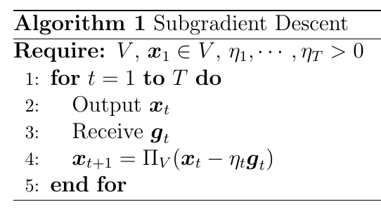
Subgradient descent (SD) is a very simple algorithm for minimizing a non-differentiable convex function. It proceeds iteratively updating the vector ${{\boldsymbol x}_t}$ moving in the direction of a negative subgradient ${{\boldsymbol g}_t}$ , but a positive factor ${\eta_t}$ called the stepsize. Also, we project onto the feasible set ${V}$ . The pseudocode is in Algorithm 1. It is similar to the gradient descent algorithm, but it has some important conceptual differences.

algo_sd

First, here, we do not assume differentiability of the function so we only have access to a subgradient ${{\boldsymbol g}}$ in any point ${{\boldsymbol x}_0}$ in ${V}$ , i.e. ${{\boldsymbol g} \in \partial f({\boldsymbol x}_0)}$ . Note that this situation is more common than one would think. For example, the hinge loss, ${f({\boldsymbol w})=\max(1-y\langle {\boldsymbol w},{\boldsymbol x}\rangle,0)}$ , and the ReLU activation function used in neural networks, ${f(x)=\max(x,0)}$ , are not differentiable.

A second difference, is that SD is not a descent method, that is, it can happen that ${f({\boldsymbol x}_{t+1})>f({\boldsymbol x}_t)}$ . The objective function can stay the same or even increase over iterates, no matter what stepsize is used. In fact, a common misunderstanding is that in SD methods the subgradient tells us in which direction to go in order to decrease the value of the function. This wrong intuition often comes from thinking about one dimensional functions. Also, this makes the choice of the stepsizes critical to obtain convergence.

Let’s analyze these issues one at the time.

Subgradient. Let’s first define formally what is a subgradient. For a function ${f:{\mathbb R}^d \rightarrow {\mathbb R}}$ , we define a subgradient of ${f}$ in ${{\boldsymbol x} \in {\mathbb R}^d}$ as a vector ${{\boldsymbol g} \in {\mathbb R}^d}$ that satisfies

$\displaystyle f({\boldsymbol y})\geq f({\boldsymbol x}) + \langle {\boldsymbol g}, {\boldsymbol y}-{\boldsymbol x}\rangle, \ \forall {\boldsymbol y} \in {\mathbb R}^d~.$

Basically, a subgradient of ${f}$ in ${{\boldsymbol x}}$ is any vector ${{\boldsymbol g}}$ that allows us to construct a linear lower bound to ${f}$ . Note that the subgradient is not unique, so we denote the set of subgradients of ${f}$ in ${{\boldsymbol x}}$ by ${\partial f({\boldsymbol x})}$ . If the function is convex, differentiable in ${{\boldsymbol x}}$ , and ${f}$ is finite in ${{\boldsymbol x}}$ , we have that the subdifferential is composed by a unique element equal to ${\nabla f({\boldsymbol x})}$ (Rockafellar, R. T., 1970)[Theorem 25.1].

Now, we can take a look at the following examples that illustrate the fact that a subgradient does not always point in a direction where the function decreases.

Example 1

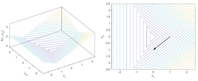
Figure 1. 3D plot (left) and level sets (right) of ${f(\boldsymbol x)=\max[-x_1,x_1-x_2,x_1+x_2]}$ . The negative subgradient is indicated by the black arrow.
Figure 2. 3D plot (left) and level sets (right) of ${f(\boldsymbol x)=\max[x_1^2+(x_2+1)^2,x_1^2+(x_2-1)^2]}$ . The negative subgradient is indicated by the black arrow.
Let ${f({\boldsymbol x})=\max[-x_1,x_1-x_2,x_1+x_2]}$ , see Figure 1. The vector ${{\boldsymbol g}=[1,1]}$ is a subgradient in ${{\boldsymbol x}=(1,0)}$ of ${f({\boldsymbol x})}$ . No matter how we choose the stepsize, moving in the direction of the negative subgradient will not decrease the objective function. An even more extreme example is in Figure 2, with the function ${f({\boldsymbol x})=\max[x_1^2+(x_2+1)^2,x_1^2+(x_2-1)^2]}$ . Here, in the point ${(1,0)}$ , any positive step in the direction of the negative subgradient will increase the objective function.

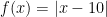
Another effect of the fact that the objective function is non-differentiable is that we cannot use a constant stepsize. This is easy to visualize, even for one-dimensional functions. Take a look for example at the function ${f(x)=|x-10|}$ in Figure 3(left). For any fixed stepsize and any number of iterations, we will never converge to the minimum of the function. Hence, if you want to converge to the minimum, you must use a decreasing stepsize. The same does not happen for smooth functions, for example ${f(x)=\frac{1}{10}(x-10)^2}$ in Figure 3(right), where the same constant stepsize gives rise to an automatic slowdown in the vicinity of the minimum, because the magnitude of the gradient decreases.

sd_stepsizes — Figure 3. The effect of a constant stepsize on non-differentiable (left) and smooth (right) functions.

Reintepreting the Subgradient Descent Algorithm. Given that SD does not work because it moves towards the minimum, let’s see how it actually works. So, first we have to correctly interpret its behavior.

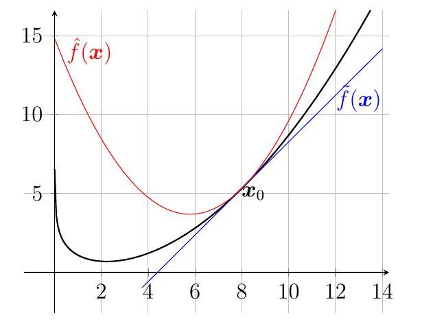
A way to understand how SD algorithms work is to think that they minimize a local approximation of the original objective function. This is not unusual for optimization algorithms, for example the Netwon’s algorithm construct an approximation with a Taylor expansion truncated to the second term. Thanks to the definition of subgradients, we can immediately build a linear lower bound to the function around ${{\boldsymbol x}_0}$ :

$\displaystyle f({\boldsymbol x}) \geq \tilde{f}({\boldsymbol x}) := f({\boldsymbol x}_0) + \langle {\boldsymbol g}, {\boldsymbol x}-{\boldsymbol x}_0\rangle, \ \forall {\boldsymbol x} \in V~.$

Unfortunately, minimizing a linear function is unlikely to give us a good optimization algorithm. Indeed, over unbounded domains the minimum of a linear function can be ${-\infty}$ . Hence, the intuitive idea is to constraint the minimization of this lower bound only in a neighboorhood of ${{\boldsymbol x}_t}$ , where we know that the approximation is more precise. Coding the neighboorhood constraint with a L2 squared distance from ${{\boldsymbol x}_t}$ less than some positive number ${h}$ , we might think to use the following update

$\displaystyle \begin{aligned} {\boldsymbol x}_{t+1} = \mathop{\text{argmin}}_{{\boldsymbol x} \in V} & \ f({\boldsymbol x}_t) + \langle {\boldsymbol g}_t, {\boldsymbol x}-{\boldsymbol x}_t\rangle \\ \text{s.t.} & \ \|{\boldsymbol x}_t-{\boldsymbol x}\|^2 \leq h~. \end{aligned}$

Equivalently, for some ${\eta>0}$ , we can consider the unconstrained formulation

$\displaystyle \label{eq:quad_approx} {\boldsymbol x}_{t+1} = \mathop{\text{argmin}}_{{\boldsymbol x} \in V} \ \hat{f}({\boldsymbol x}):=f({\boldsymbol x}_t) + \langle {\boldsymbol g}_t, {\boldsymbol x}-{\boldsymbol x}_t\rangle + \frac{1}{2\eta}\|{\boldsymbol x}_{t}-{\boldsymbol x}\|_2^2~. \ \ \ \ \ (1)$

This is a well-defined update scheme, that hopefully moves ${{\boldsymbol x}_t}$ closer to the optimum of ${f}$ . See Figure 4 for a graphical representation in one-dimension.

sd_approximations — Figure 4. Approximations of ${f({\boldsymbol x})}$ .

Figure 4. Approximations of ${f({\boldsymbol x})}$ .

sd_algo2

Solving the argmin and completing the square, we get

$\displaystyle \begin{aligned} \mathop{\text{argmin}}_{{\boldsymbol x} \in V} \ \langle {\boldsymbol g}_t, x\rangle + \frac{1}{2\eta_t}\|{\boldsymbol x}_{t}-{\boldsymbol x}\|_2^2 &= \mathop{\text{argmin}}_{{\boldsymbol x} \in V} \ \|\eta_t {\boldsymbol g}_t\|^2 + 2\eta_t \langle {\boldsymbol g}_t, x-{\boldsymbol x}_t\rangle + \|{\boldsymbol x}_{t}-{\boldsymbol x}\|_2^2 \\ &= \mathop{\text{argmin}}_{{\boldsymbol x} \in V} \ \|{\boldsymbol x}_t -\eta_t {\boldsymbol g}_t -{\boldsymbol x}\|_2^2 \\ &= \Pi_V({\boldsymbol x}_t - \eta_t {\boldsymbol g}_t), \end{aligned}$

where ${\Pi_V}$ is the Euclidean projection onto ${V}$ , i.e. ${\Pi_V({\boldsymbol x})=\mathop{\text{argmin}}_{{\boldsymbol y} \in V} \|{\boldsymbol x}-{\boldsymbol y}\|_2}$ . This is exactly the update of SD in Algorithm 1.

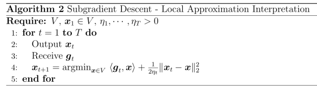
However, we can also obtain a different closed form update. Ignoring the constant term with respect to ${{\boldsymbol x}}$ , from (1) we obtain the update step of SD in Algorithm 2. This will be useful when we will extend subgradient descent to different norms than L2.

Convergence Analysis. We have shown how to correctly intepret SD. Yet, its intepretation is not a proof of its convergence. Indeed, the interpretation above does not say anything about the stepsizes. So, here we will finally show its convergence guarantee.

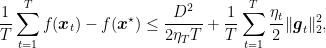
We can now show the convergence guarantee for SD. In particular we want to show that

$\displaystyle f({\boldsymbol x}_T)-f({\boldsymbol x}^\star) \leq O\left(\frac{1}{\sqrt{T}}\right),$

that is optimal for this setting. Keeping in mind that SD is not a descent method, the proof of convergence cannot aim at proving that at each step we descrease the function by a minimum amount. Instead, we show that the suboptimality gap at each step is upper bounded by a term, whose sum grows sublinearly. This means, that the average, and so the minimum, of the suboptimality gaps decreases with the number of iterations.

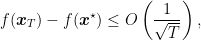
First, we show the following two Lemmas. The first lemma proves that Euclidean projections always decrease the distance with points inside the set.

Proposition 1 Let ${{\boldsymbol x} \in {\mathbb R}^d}$ and ${{\boldsymbol y} \in V}$ , where ${V \subset {\mathbb R}^d}$ is a closed convex set. Then, ${\|\Pi_V({\boldsymbol x})-{\boldsymbol y}\|_2 \leq \|{\boldsymbol x}-{\boldsymbol y}\|_2}$ .

Proof: By the convexity of ${V}$ , we have that
${\Pi_V({\boldsymbol x})+ \alpha ({\boldsymbol y}-\Pi_V({\boldsymbol x})) \in V}$ for all ${0 \leq \alpha \leq 1}$ . Hence, from the optimality of ${\Pi_V({\boldsymbol x})}$ , we have

$\displaystyle \begin{aligned} \|\Pi_V({\boldsymbol x})-{\boldsymbol x}\|_2^2 &\leq \left\|\Pi_V({\boldsymbol x})+\alpha ({\boldsymbol y}-\Pi_V({\boldsymbol x}))-{\boldsymbol x}\right\|_2^2 \\ &= \|\Pi_V({\boldsymbol x})-{\boldsymbol x}\|^2_2 + 2 \alpha \langle \Pi_V({\boldsymbol x})-{\boldsymbol x}, {\boldsymbol y}-\Pi_V({\boldsymbol x})\rangle +\alpha^2 \|{\boldsymbol y}-\Pi_V({\boldsymbol x})\|_2^2~. \end{aligned}$

Rearranging, we obtain

$\displaystyle 2 \langle \Pi_V({\boldsymbol x})-{\boldsymbol x}, {\boldsymbol y}-\Pi_V({\boldsymbol x})\rangle \geq -\alpha \|{\boldsymbol y}-\Pi_V({\boldsymbol x})\|_2^2~.$

Taking the limit ${\alpha\rightarrow 0}$ , we get that

$\displaystyle \langle \Pi_V({\boldsymbol x})-{\boldsymbol x}, {\boldsymbol y}-\Pi_V({\boldsymbol x})\rangle \geq 0~.$

Therefore,

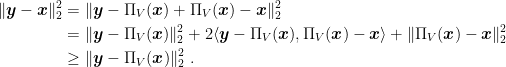
$\displaystyle \begin{aligned} \|{\boldsymbol y} - {\boldsymbol x}\|_2^2 &= \|{\boldsymbol y}-\Pi_V({\boldsymbol x})+\Pi_V({\boldsymbol x})-{\boldsymbol x}\|_2^2 \\ &= \|{\boldsymbol y}-\Pi_V({\boldsymbol x})\|^2_2 +2 \langle {\boldsymbol y}-\Pi_V({\boldsymbol x}),\Pi_V({\boldsymbol x})-{\boldsymbol x}\rangle + \|\Pi_V({\boldsymbol x})-{\boldsymbol x}\|_2^2 \\ &\geq \|{\boldsymbol y}-\Pi_V({\boldsymbol x})\|_2^2~. \end{aligned}$

$\Box$

The next lemma upper bounds the suboptimality gap in one iteration.

Lemma 2 Let ${V\subset {\mathbb R}^d}$ a closed non-empty convex set and ${f}$ a convex function from ${V\subseteq {\mathbb R}^d}$ to ${{\mathbb R}}$ . Set ${{\boldsymbol g}_t \in \partial f({\boldsymbol x}_t)}$ . Then, ${\forall {\boldsymbol u} \in V}$ , the following inequality holds

$\displaystyle \eta_t (f({\boldsymbol x}_t)- f({\boldsymbol u}) ) \leq \eta_t \langle {\boldsymbol g}_t, {\boldsymbol x}_t -{\boldsymbol u}\rangle \leq \frac{1}{2}\|{\boldsymbol x}_t-{\boldsymbol u}\|^2_2 - \frac{1}{2}\|{\boldsymbol x}_{t+1}-{\boldsymbol u}\|^2_2 + \frac{\eta_t^2}{2}\|{\boldsymbol g}_t\|_2^2~.$

Proof: From Proposition 1 and the definition of subgradient, we have that

$\displaystyle \begin{aligned} \|{\boldsymbol x}_{t+1}-{\boldsymbol u}\|^2_2 - \|{\boldsymbol x}_{t}-{\boldsymbol u}\|^2_2 &\leq \|{\boldsymbol x}_t-\eta_t {\boldsymbol g}_t -{\boldsymbol u}\|^2_2 - \|{\boldsymbol x}_{t}-{\boldsymbol u}\|^2_2 \\ &= -2 \eta_t \langle {\boldsymbol g}_t, {\boldsymbol x}_t - {\boldsymbol u}\rangle + \eta_t^2 \|{\boldsymbol g}_t\|^2_2 \\ &\leq -2 \eta_t (f({\boldsymbol x}_t) - f({\boldsymbol u})) + \eta_t^2 \|{\boldsymbol g}_t\|^2_2~. \end{aligned}$

Reordering, we have the stated bound. $\Box$

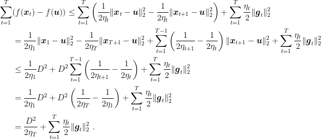
Theorem 3 Let ${V\subset {\mathbb R}^d}$ a closed non-empty convex set with diameter ${D}$ , i.e. ${\max_{{\boldsymbol x},{\boldsymbol y}\in V} \|{\boldsymbol x}-{\boldsymbol y}\| \leq D}$ . Let ${f}$ a convex function from ${V\subseteq {\mathbb R}^d}$ to ${{\mathbb R}}$ . Set ${{\boldsymbol x}_1 \in V}$ . Set ${{\boldsymbol g}_t \in \partial f({\boldsymbol x}_t)}$ . Then, ${\forall {\boldsymbol u} \in V}$ , the following convergence bound hold

$\displaystyle \begin{aligned} f\left(\frac{1}{T}\sum_{t=1}^T {\boldsymbol x}_t\right) - f({\boldsymbol x}^\star) &\leq \frac{\frac{D^2}{\eta_{T}} + \sum_{t=1}^T \eta_t \|{\boldsymbol g}_t\|^2_2}{2T},\\ f\left(\frac{\sum_{t=1}^T \eta_t {\boldsymbol x}_t}{\sum_{t=1}^T \eta_t}\right) - f({\boldsymbol x}^\star) &\leq \frac{\|{\boldsymbol x}_1-{\boldsymbol u}\|^2_2 + \sum_{t=1}^T \eta_t^2\|{\boldsymbol g}_t\|^2_2}{2\sum_{t=1}^T \eta_t},\\ \min_{1 \leq t\leq T} f\left({\boldsymbol x}_t\right) - f({\boldsymbol x}^\star) &\leq \min\left(\frac{\frac{D^2}{\eta_{T}} + \sum_{t=1}^T \eta_t \|{\boldsymbol g}_t\|^2_2}{2T},\frac{\|{\boldsymbol x}_1-{\boldsymbol u}\|^2_2 + \sum_{t=1}^T \eta_t^2\|{\boldsymbol g}_t\|^2_2}{2\sum_{t=1}^T \eta_t}\right)~. \end{aligned}$

Proof: Dividing the inequality in Lemma 2 by ${2\eta_t}$ and summing over ${t=1,\cdots,T}$ , we have

$\displaystyle \begin{aligned} \sum_{t=1}^T &(f({\boldsymbol x}_t) - f({\boldsymbol u})) \leq \sum_{t=1}^T \left(\frac{1}{2\eta_t}\|{\boldsymbol x}_{t}-{\boldsymbol u}\|^2_2 - \frac{1}{2\eta_t}\|{\boldsymbol x}_{t+1}-{\boldsymbol u}\|^2_2\right) + \sum_{t=1}^T \frac{\eta_t}{2} \|{\boldsymbol g}_t\|^2_2 \\ &= \frac{1}{2\eta_1}\|{\boldsymbol x}_{1}-{\boldsymbol u}\|^2_2 - \frac{1}{2\eta_T} \|{\boldsymbol x}_{T+1}-{\boldsymbol u}\|^2_2 + \sum_{t=1}^{T-1} \left(\frac{1}{2\eta_{t+1}}-\frac{1}{2\eta_t}\right)\|{\boldsymbol x}_{t+1}-{\boldsymbol u}\|^2_2 + \sum_{t=1}^T \frac{\eta_t}{2} \|{\boldsymbol g}_t\|^2_2 \\ &\leq \frac{1}{2\eta_1} D^2 + D^2 \sum_{t=1}^{T-1} \left(\frac{1}{2\eta_{t+1}}-\frac{1}{2\eta_{t}}\right) + \sum_{t=1}^T \frac{\eta_t}{2} \|{\boldsymbol g}_t\|^2_2 \\ &= \frac{1}{2\eta_1} D^2 + D^2 \left(\frac{1}{2\eta_{T}}-\frac{1}{2\eta_1}\right) + \sum_{t=1}^T \frac{\eta_t}{2} \|{\boldsymbol g}_t\|^2_2 \\ &= \frac{D^2}{2\eta_{T}} + \sum_{t=1}^T \frac{\eta_t}{2} \|{\boldsymbol g}_t\|^2_2~. \end{aligned}$

Dividing both terms by ${T}$ , we have

$\displaystyle \frac{1}{T}\sum_{t=1}^T f({\boldsymbol x}_t) - f({\boldsymbol x}^\star) \leq \frac{D^2}{2\eta_{T}T} + \frac{1}{T}\sum_{t=1}^T \frac{\eta_t}{2} \|{\boldsymbol g}_t\|^2_2,$

This is almost a convergence rate, but we need to extract one of the ${{\boldsymbol x}_t}$ in some way. Hence, we just use Jensen’s inequality on the lhs.

For the second statement, consider the inequality in Lemma 2, divide both sides by 2, and sum over ${t=1,\cdots,T}$ .

$\displaystyle \begin{aligned} \sum_{t=1}^T \eta_t (f({\boldsymbol x}_t) - f({\boldsymbol x}^\star)) &\leq \sum_{t=1}^T \left(\frac{1}{2}\|{\boldsymbol x}_{t}-{\boldsymbol u}\|^2_2 - \frac{1}{2}\|{\boldsymbol x}_{t+1}-{\boldsymbol u}\|^2_2\right) + \frac{1}{2}\sum_{t=1}^T \eta_t^2\|{\boldsymbol g}_t\|^2_2 \\ &= \frac{1}{2}\|{\boldsymbol x}_1-{\boldsymbol u}\|^2_2 - \frac{1}{2}\|{\boldsymbol x}_{T+1}-{\boldsymbol u}\|^2_2 + \frac{1}{2}\sum_{t=1}^T \eta_t^2 \|{\boldsymbol g}_t\|^2_2 \\ &\leq \frac{1}{2}\|{\boldsymbol x}_1-{\boldsymbol u}\|^2_2 + \frac{1}{2}\sum_{t=1}^T \eta_t^2 \|{\boldsymbol g}_t\|^2_2~. \end{aligned}$

Then, again use Jensen’s inequality.

For the third statement, use the fact that

$\displaystyle \left( \min_{1 \leq t\leq T} f({\boldsymbol x}_t) - f({\boldsymbol x}^\star)\right)\sum_{i=1}^T a_i \leq \sum_{t=1}^T a_i (f({\boldsymbol x}_t)-f({\boldsymbol x}^\star)), \ \forall a_i\geq0~.$

$\Box$

We can immediately observe few things. First, the most known convergence bound for SD (first bound in the theorem) need a bounded domain ${V}$ . In most of the machine learning applications, this assumptions is false. In general, we should be very worried when we use a theorem whose assumptions are clearly false. It is like using a new car that is guaranteed to work only when the outside temperature is above 68 Degrees Fahrenheit, and in the other cases “it seems to work, but we are not sure about it”. Would you drive it?
So, for unbounded domains, we have to rely on the lesser-known second and third guarantees, see, e.g., Zhang, T. (2004).

The other observation is that the above guarantees do not justify the common heuristic of taking the last iterate. Indeed, as we said, SD is not a descent method so the last iterate is not guaranteed to be best one. In the following posts, we will see that we can still prove that the last iterate converges, even in the unbounded case, but the convergence rate gets an additional logarithmic factor.

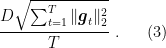
Another important observation is to use the convergence guarantee to choose the stepsizes. Indeed, it is the only guideline we have. Any other choice that is not justified by a convergence analysis it is not justified at all. A simple choice is to find the constant stepsize that minimizes the bounds for a fixed number of iterations. For simplicity, let’s assume that the domain is bounded. So, in all cases, we have to consider the expression

$\displaystyle \frac{D^2}{2\eta} + \frac{\eta}{2} \sum_{t=1}^T \|{\boldsymbol g}_t\|_2^2$

and minimize with respect to ${\eta}$ . It is easy to see that the optimal ${\eta}$ is ${\frac{D}{\sqrt{\sum_{t=1}^T \|{\boldsymbol g}_t\|_2^2}}}$ . See how that gives the regret bound

$\displaystyle \label{eq:md_opt_regret} D\sqrt{\sum_{t=1}^T \|{\boldsymbol g}_t\|_2^2} \ \ \ \ \ (2)$

and the convergence rate

$\displaystyle \label{eq:md_opt_convergence} \frac{D\sqrt{\sum_{t=1}^T \|{\boldsymbol g}_t\|_2^2}}{T}~. \ \ \ \ \ (3)$

However, we have a problem: in order to use this stepsize, we should know the future subgradients! This is exactly the core idea of adaptive algorithms: how the obtain the best possible guarantee without knowning impossible quantities?

We will see many adaptive strategies, but, for the moment, we can observe that we might be happy to minimize a looser upper bound. In particular, assuming that the functions are ${L}$ -Lischtiz, we have that ${\|{\boldsymbol g}_t\|_2 \leq L}$ . Hence, we have

$\displaystyle \eta^\star = \mathop{\text{argmin}}_\eta \frac{D^2}{2\eta} + \frac{\eta L^2 T}{2} = \frac{D}{L \sqrt{T}},$

that gives a convergence rate of ${\frac{D L}{\sqrt{T}}}$ .

5 Comments

Pingback: The Negative Gradient Does Not Point Towards the Minimum – Parameter-free Learning and Optimization Algorithms
Pingback: Online Mirror Descent I: Bregman version – Parameter-free Learning and Optimization Algorithms
Max says:

October 2, 2019 at 9:03 AM

Thanks for the nice explanations. If you don’t mind me asking as silly question. In algorithm 2 in the step of completing the square and solving argmin is there a missing negative (eta_t*gt)^2 term? Shouldn’t we keep the balance when completing the square? (ax^2+bx = x^2+bxa/2+(bxa/2)^2-(bxa/2)^2)? Thanks

LikeLike

1. bremen79 says:
  
  October 2, 2019 at 10:16 AM
  
  Hi Max, sure you could keep that term around, but the argmin would not change because it does not depend on x. Indeed, the argmin is the position of the minimum that does not change if you add a constant term to the function.
  
  LikeLike
  
Max says:

October 4, 2019 at 7:31 AM

Grazie mille, Francesco for the clarification.

LikeLiked by 1 person

Pingback: Last Iterate of SGD Converges (Even in Unbounded Domains) – Parameter-free Learning and Optimization Algorithms
Denizap Goktas says:

October 7, 2020 at 7:28 PM

Hi Professor Orabona,
Thank you for this page! I would like to cite the results on this post, is there any paper I could refer to? I can’t seem to find these results anywhere else.

LikeLike

1. bremen79 says:
  
  October 7, 2020 at 8:40 PM
  
  Hi Denizap, I am glad you liked this post!
  The fact that subgradient descent is not a descent method I guess it is a known result in convex optimization, I am not even sure where I read it for the first time. But if you want a citation, you can cite my monograph on online learning: https://arxiv.org/pdf/1912.13213.pdf You can find the negative examples on this page in Section 6.1 and the theorems in Chapter 6. It is online learning rather than batch, but the theorems are the same. There you can also find the correct citations.
  
  LikeLike
  
Pingback: Implicit, Passive-Aggressive, and aProx updates – Parameter-free Learning and Optimization Algorithms