Online Mirror Descent II: Regret and Mirror Version

This post is part of the lecture notes of my class “Introduction to Online Learning” at Boston University, Fall 2019. I will publish two lectures per week.

You can find the lectures I published till now here.


1. Online Mirror Descent

omd

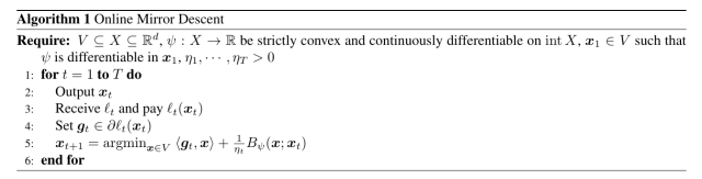
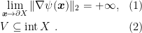
Last time we introduced the Online Mirror Descent (OMD) algorithm, in Algorithm 1. We also said that we need one of these two assumptions to hold.

\displaystyle \begin{aligned} &\lim_{{\boldsymbol x} \rightarrow \partial X} \|\nabla \psi({\boldsymbol x})\|_2 = +\infty, & (1) \\ &V\subseteq \mathop{\mathrm{int}} X~. & (2) \\\end{aligned}

We also proved the following Lemma.

Lemma 1 Let {B_\psi} the Bregman divergence w.r.t. {\psi: X \rightarrow {\mathbb R}} and assume {\psi} to be {\lambda}-strongly convex with respect to {\|\cdot\|} in {V}. Let {V \subseteq X} a closed convex set. Set {{\boldsymbol g}_t \in \partial \ell_t({\boldsymbol x}_t)}. Assume (1) or (2) hold. Then, {\forall {\boldsymbol u} \in V} and with the notation in Algorithm 1, the following inequality holds

\displaystyle \eta_t (\ell_t({\boldsymbol x}_t) - \ell_t({\boldsymbol u}) ) \leq \eta_t \langle {\boldsymbol g}_t, {\boldsymbol x}_t -{\boldsymbol u}\rangle \leq B_\psi({\boldsymbol u};{\boldsymbol x}_t) - B_\psi({\boldsymbol u};{\boldsymbol x}_{t+1}) + \frac{\eta_t^2}{2\lambda}\|{\boldsymbol g}_t\|_\star^2~.

Today, we will finally prove a regret bound for OMD.
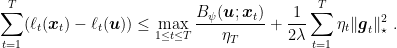
Theorem 2 Set {{\boldsymbol x}_1 \in V} such that {\psi} is differentiable in {{\boldsymbol x}_1}. Assume {\eta_{t+1}\leq \eta_{t}, \ t=1, \dots, T}. Then, under the assumptions of Lemma 1 and {\forall {\boldsymbol u} \in V}, the following regret bounds hold

\displaystyle \sum_{t=1}^T (\ell_t({\boldsymbol x}_t)- \ell_t({\boldsymbol u})) \leq \max_{1\leq t \leq T} \frac{B_\psi({\boldsymbol u};{\boldsymbol x}_t)}{\eta_{T}} + \frac{1}{2\lambda}\sum_{t=1}^T \eta_t \|{\boldsymbol g}_t\|^2_\star~.

Moreover, if {\eta_t} is constant, i.e. {\eta_t=\eta \ \forall t=1,\cdots,T}, we have

\displaystyle \sum_{t=1}^T (\ell_t({\boldsymbol x}_t)- \ell_t({\boldsymbol u})) \leq \frac{B_\psi({\boldsymbol u};{\boldsymbol x}_1)}{\eta} + \frac{\eta}{2\lambda}\sum_{t=1}^T \|{\boldsymbol g}_t\|^2_\star~.

Proof: Fix {{\boldsymbol u} \in V}. As in the proof of OGD, dividing the inequality in Lemma 1 by {\eta_t} and summing from {t=1,\cdots,T}, we get

\displaystyle \begin{aligned} \sum_{t=1}^T &(\ell_t({\boldsymbol x}_t) - \ell_t({\boldsymbol u})) \leq \sum_{t=1}^T \left(\frac{1}{\eta_t}B_\psi({\boldsymbol u};{\boldsymbol x}_t) - \frac{1}{\eta_t}B_\psi({\boldsymbol u};{\boldsymbol x}_{t+1})\right) + \sum_{t=1}^T \frac{\eta_t}{2\lambda} \|{\boldsymbol g}_t\|^2_\star \\ &= \frac{1}{\eta_1}B_\psi({\boldsymbol u};{\boldsymbol x}_{1}) - \frac{1}{\eta_T} B_\psi({\boldsymbol u};{\boldsymbol x}_{T+1}) + \sum_{t=1}^{T-1} \left(\frac{1}{\eta_{t+1}}-\frac{1}{\eta_t}\right)B_\psi({\boldsymbol u};{\boldsymbol x}_{t+1}) + \sum_{t=1}^T \frac{\eta_t}{2\lambda} \|{\boldsymbol g}_t\|^2_\star \\ &\leq \frac{1}{\eta_1} D^2 + D^2 \sum_{t=1}^{T-1} \left(\frac{1}{\eta_{t+1}}-\frac{1}{\eta_{t}}\right) + \sum_{t=1}^T \frac{\eta_t}{2\lambda} \|{\boldsymbol g}_t\|^2_\star \\ &= \frac{1}{\eta_1} D^2 + D^2 \left(\frac{1}{\eta_{T}}-\frac{1}{\eta_1}\right) + \sum_{t=1}^T \frac{\eta_t}{2} \|{\boldsymbol g}_t\|^2_\star \\ &= \frac{D^2}{\eta_{T}} + \sum_{t=1}^T \frac{\eta_t}{2\lambda} \|{\boldsymbol g}_t\|^2_\star, \end{aligned}

where we denoted by {D^2=\max_{1\leq t\leq T} B_\psi({\boldsymbol u};{\boldsymbol x}_t)}.

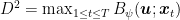
The second statement is left as an exercise. \Box

In words, OMD allows us to prove regret guarantees that depend on arbitrary couple of dual norms {\|\cdot\|} and {\|\cdot\|_\star}. In particular, the primal norm will be used to measure the feasible set {V} or the distance between the competitor and the initial point, and the dual norm will be used to measure the gradients. If you happen to know something about these quantities, we can choose the most appropriate couple of norm to guarantee a small regret. The only thing you need is a function {\psi} that is strongly convex with respect to the primal norm you have chosen {\psi}.

Overall, the regret bound is still of the order of {\sqrt{T}} for Lipschitz functions, that only difference is that now the Lipschitz constant is measured with a different norm. Also, everything we did for Online Subgradient Descent (OSD) can be trivially used here. So, for example, we can use stepsize of the form

\displaystyle \eta_t=\frac{D \sqrt{\lambda}}{\sqrt{\sum_{i=1}^t \|{\boldsymbol g}_i\|_*^2}}

to achieve a regret bound of {2 \frac{D}{\sqrt{\lambda}} \sqrt{\sum_{t=1}^T \|{\boldsymbol g}_t\|^2_\star}}.

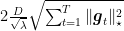
Next time, we will see practical examples of OMD that guarantee strictly better regret than OSD. As we did in the case of AdaGrad, the better guarantee will depend on the shape of the domain and the characteristics of the subgradients.

Instead, now we see the meaning of the “Mirror”.

2. The “Mirror” Interpretation

First, we need a couple of convex analysis results.

When we introduced the Fenchel conjugate, we said that {{\boldsymbol x} \in \partial f^\star({\boldsymbol \theta})} iff {{\boldsymbol \theta} \in \partial f({\boldsymbol x})}, that in words means that {(\partial f)^{-1} = \partial f^\star} in the sense of multivalued mappings. Now, we state a stronger result for the case that the function is strongly convex.

Theorem 3 Let {\psi:{\mathbb R}^d \rightarrow (-\infty, +\infty]} be a proper, convex, and closed function, {\lambda>0} strongly convex w.r.t. {\|\cdot\|}. Then,

  1. {\psi^\star} is finite everywhere and differentiable.
  2. {\psi^\star} is {\frac{1}{\lambda}}-smooth w.r.t. {\|\cdot\|_\star}.

We will also use the following optimality condition.

Theorem 4 Let {f: {\mathbb R}^d \rightarrow (-\infty, +\infty]} proper. Then {{\boldsymbol x}^\star \in \mathop{\mathrm{argmin}}_{{\boldsymbol x} \in {\mathbb R}^d} f({\boldsymbol x})} iff {\boldsymbol{0} \in \partial f({\boldsymbol x}^\star)}.

Hence, we can state the following theorem.

Theorem 5 Let {B_\psi} the Bregman divergence w.r.t. {\psi: X \rightarrow {\mathbb R}}, where {\psi} is {\lambda>0} strongly convex. Let {V \subseteq X} a non-empty closed convex set such that {\mathop{\mathrm{int}} X \cap V \neq \{\}}. Then

\displaystyle \label{eq:mirror_update} \mathop{\mathrm{argmin}}_{{\boldsymbol x} \in V} \ \langle {\boldsymbol g}_t, {\boldsymbol x}\rangle + \frac{1}{\eta_t}B_\psi({\boldsymbol x}; {\boldsymbol x}_{t}) = \nabla \psi_V^\star( \nabla \psi_V({\boldsymbol x}_t) - \eta_t {\boldsymbol g}_t), \ \ \ \ \ (3)

where {\psi_V} the restriction of {\psi} to {V}, that is {\psi_V:=\psi + i_V}.

Proof: Consider the update rule in Algorithm 1 and let’s see

\displaystyle \begin{aligned} {\boldsymbol x}_{t+1} &= \mathop{\mathrm{argmin}}_{{\boldsymbol x} \in V} \ \langle {\boldsymbol g}_t, {\boldsymbol x}\rangle + \frac{1}{\eta_t}B_\psi({\boldsymbol x}; {\boldsymbol x}_{t}) \\ &= \mathop{\mathrm{argmin}}_{{\boldsymbol x} \in V} \ \eta_t \langle {\boldsymbol g}_t, {\boldsymbol x}\rangle + B_\psi({\boldsymbol x}; {\boldsymbol x}_{t}) \\ &= \mathop{\mathrm{argmin}}_{{\boldsymbol x} \in V} \ \eta_t \langle {\boldsymbol g}_t, {\boldsymbol x}\rangle + \psi({\boldsymbol x}) - \psi({\boldsymbol x}_{t}) -\langle \nabla \psi({\boldsymbol x}_t), {\boldsymbol x}-{\boldsymbol x}_t\rangle \\ &= \mathop{\mathrm{argmin}}_{{\boldsymbol x} \in V} \ \langle \eta_t {\boldsymbol g}_t-\nabla \psi({\boldsymbol x}_t), {\boldsymbol x}\rangle + \psi({\boldsymbol x})~. \end{aligned}

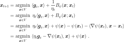
Now, we want to use the first order optimality condition, so we have to use a little bit of subdifferential calculus. Given that {\mathop{\mathrm{int}} X \cap V \neq \{\}}, by the subdifferential calculus theorem we saw, we have {\partial (f+g) = \partial f + \partial g}. So, we have

\displaystyle \boldsymbol{0} \in \eta_t {\boldsymbol g}_t + \nabla \psi ({\boldsymbol x}_{t+1}) - \nabla \psi({\boldsymbol x}_t) + \partial i_V({\boldsymbol x}_{t+1})~.

that is

\displaystyle \nabla \psi({\boldsymbol x}_t) - \eta_t {\boldsymbol g}_t \in (\nabla \psi + \partial i_V)({\boldsymbol x}_{t+1}) = \partial \psi_V({\boldsymbol x}_{t+1})~.

or equivalently

\displaystyle {\boldsymbol x}_{t+1} \in \partial \psi_V^\star(\nabla \psi({\boldsymbol x}_t) - \eta_t {\boldsymbol g}_t)~.

Using that fact that {\psi_V :=\psi + i_V} is {\lambda}-strongly convex, we have that {\partial \psi_V^\star=\{\nabla \psi_V^\star\}}. Hence

\displaystyle {\boldsymbol x}_{t+1} = \nabla \psi_V^\star( \nabla \psi({\boldsymbol x}_t) - \eta_t {\boldsymbol g}_t)~.

Noting that {\psi_V\equiv \psi} for vectors in {V}, we have the stated bound. \Box

duality maps
Figure 1. OMD update in terms of duality mappings.

Let’s explain what this theorem says. We said that Online Mirror Descent extends the Online Subgradient Descent method to non-euclidean norms. Hence, the regret bound we proved contains dual norms, that measure the iterate and the gradients. We also said that it makes sense to use a dual norm to measure a gradient, because it is a natural way to measure how “big” is the linear functional {{\boldsymbol x} \rightarrow \langle \nabla f({\boldsymbol y}), {\boldsymbol x}\rangle}. In a more correct way, gradients actually live in the dual space, that is in a different space of the predictions {{\boldsymbol x}_t}. Hence, we cannot sum iterates and gradients together, in the same way in which we cannot sum pear and apples together. So, why we were doing it in OSD? The reason is that in that case the dual space coincides with the primal space. But, it is a very particular case due to the fact that we used the L2 norm. Instead, in the general case, iterates and gradients are in two different spaces.

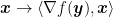
So, in OMD we need a way to go from one space to the other. And this is exactly the role of
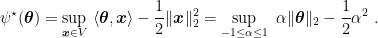
 {\nabla \psi} and {\nabla \psi^\star}, that are called duality mappings. We can now understand that the theorem tells us that OMD takes the primal vector {{\boldsymbol x}_t}, transforms it into a dual vector through {\nabla \psi}, does a subgradient descent step in the dual space, and finally transforms the vector back to the primal space through {\nabla \psi^\star}. This reasoning is summarized in Figure 1.

Example 1 Let {\psi:{\mathbb R}^d \rightarrow {\mathbb R}} equal to {\psi({\boldsymbol x})=\frac{1}{2}\|{\boldsymbol x}\|_2^2+i_V({\boldsymbol x})} where {V=\{{\boldsymbol x} \in {\mathbb R}^d: \|{\boldsymbol x}\|_2\leq 1\}}. Then,

\displaystyle \psi^\star({\boldsymbol \theta}) = \sup_{{\boldsymbol x} \in V} \ \langle {\boldsymbol \theta}, {\boldsymbol x}\rangle - \frac12 \|{\boldsymbol x}\|_2^2 = \sup_{-1 \leq \alpha\leq 1} \ \alpha \|{\boldsymbol \theta}\|_2 - \frac12 \alpha^2~.

Solving the constrained optimization problem, we have {\alpha^\star = \min(1,\|\theta\|_2)}. Hence, we have

\displaystyle \psi^\star({\boldsymbol \theta}) = \min\left(\frac{1}{2}\|{\boldsymbol \theta}\|^2_2, \|{\boldsymbol \theta}\|_2-\frac{1}{2}\right),

that is finite everywhere and differentiable. So, we have {\nabla \psi({\boldsymbol x})={\boldsymbol x}} and

\displaystyle \nabla \psi^\star({\boldsymbol \theta}) = \begin{cases} {\boldsymbol \theta}, & \|{\boldsymbol \theta}\|_2\leq 1\\ \frac{{\boldsymbol \theta}}{\|{\boldsymbol \theta}\|_2}, & \|{\boldsymbol \theta}\|_2> 1\\ \end{cases} = \Pi_V({\boldsymbol \theta})~.

So, using (3), we obtain exactly the update of projected online subgradient descent.

3. Yet Another Way to Write the OMD Update

There exists yet another way to write the update of OMD. This third method uses the concept of Bregman projections. Extending the definition of Euclidean projections, we can define the projection with respect to a Bregman divergence. Let {\Pi_{V,\psi}} be defined by

\displaystyle \Pi_{V,\psi} ({\boldsymbol x}) = \mathop{\mathrm{argmin}}_{{\boldsymbol y} \in V} \ B_\psi ({\boldsymbol y}; {\boldsymbol x})~.

In the online learning literature, the OMD algorithm is typically presented with a two step update: first, solving the argmin over the entire space and then projecting back over {X} with respect to the Bregman divergence. In the following, we show that most of the time the two-step update is equivalent to the one-step update in (3).

First, we prove a general theorem that allows to break the constrained minimization of functions in the minimization over the entire space plus and Bregman projection step.

Theorem 6 Let {f : {\mathbb R}^d \rightarrow (-\infty, +\infty]} proper, closed, strictly convex, and differentiable in {\mathop{\mathrm{int}} \mathop{\mathrm{dom}} f}. Also, let {V \subset {\mathbb R}^d} a non-empty, closed convex set with {V \cap \mathop{\mathrm{dom}} f \neq \{\}} and assume that {\tilde{{\boldsymbol y}} = \mathop{\mathrm{argmin}}_{{\boldsymbol z} \in {\mathbb R}^d} f({\boldsymbol z})} exists and {\tilde{{\boldsymbol y}} \in \mathop{\mathrm{int}} \mathop{\mathrm{dom}} f}. Denote by {{\boldsymbol y}'=\mathop{\mathrm{argmin}}_{{\boldsymbol z} \in V} B_f({\boldsymbol z}; \tilde{{\boldsymbol y}})}. Then the following hold:

  1. {{\boldsymbol y} = \mathop{\mathrm{argmin}}_{{\boldsymbol z} \in V} f({\boldsymbol z})} exists and is unique.
  2. {{\boldsymbol y} = {\boldsymbol y}'}.

Proof: For the first point, from (Bauschke, H. H. and Combettes, P. L., 2011, Proposition 11.12) and the existence of {\tilde{{\boldsymbol y}}}, we have that {f} is coercive. So, from (Bauschke, H. H. and Combettes, P. L., 2011, Proposition 11.14), the minimizer of {f} in {V} exists. Given that {f} is strictly convex, the minimizer must be unique too.

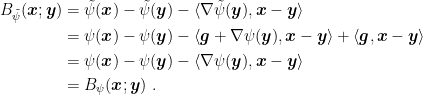
For the second point, from the definition of {{\boldsymbol y}}, we have {f({\boldsymbol y})\leq f({\boldsymbol y}')}. On the other hand, from the first-order optimality condition, we have {\nabla f(\tilde{{\boldsymbol y}}) = \boldsymbol{0}}. So, we have

\displaystyle \begin{aligned} f({\boldsymbol y}')-f(\tilde{{\boldsymbol y}}) =B_f({\boldsymbol y}'; \tilde{{\boldsymbol y}}) \leq B_f({\boldsymbol y}; \tilde{{\boldsymbol y}}) = f({\boldsymbol y}) - f(\tilde{{\boldsymbol y}}), \end{aligned}

that is {f({\boldsymbol y}')\leq f({\boldsymbol y})}. Given that {f} is strictly convex, {{\boldsymbol y}'={\boldsymbol y}}. \Box

Now, note that, if {\tilde{\psi} ({\boldsymbol x}) =\psi({\boldsymbol x}) + \langle {\boldsymbol g}, {\boldsymbol x}\rangle}, then

\displaystyle \begin{aligned} B_{\tilde{\psi}}({\boldsymbol x};{\boldsymbol y}) &= \tilde{\psi}({\boldsymbol x}) - \tilde{\psi}({\boldsymbol y}) -\langle \nabla \tilde{\psi}({\boldsymbol y}), {\boldsymbol x}-{\boldsymbol y}\rangle \\ &= \psi({\boldsymbol x}) - \psi({\boldsymbol y}) -\langle {\boldsymbol g} + \nabla \psi({\boldsymbol y}), {\boldsymbol x}-{\boldsymbol y}\rangle +\langle {\boldsymbol g}, {\boldsymbol x}-{\boldsymbol y}\rangle \\ &=\psi({\boldsymbol x}) - \psi({\boldsymbol y}) -\langle \nabla \psi({\boldsymbol y}), {\boldsymbol x}-{\boldsymbol y}\rangle \\ &= B_{\psi}({\boldsymbol x};{\boldsymbol y})~. \end{aligned}

Also, defining {g({\boldsymbol x})=B_\psi({\boldsymbol x}; {\boldsymbol y})} is equal to {\psi({\boldsymbol x})+\langle {\boldsymbol z}, {\boldsymbol x}\rangle + K} for some {K \in {\mathbb R}} and {{\boldsymbol z} \in R^d}. Hence, under the assumption of the above theorem, we have that {{\boldsymbol x}_{t+1}=\mathop{\mathrm{argmin}}_{{\boldsymbol x} \in V} \ \langle {\boldsymbol g}_t, {\boldsymbol x}\rangle + \frac{1}{\eta_t} B_\psi({\boldsymbol x};{\boldsymbol x}_t)} is equivalent to

\displaystyle \begin{aligned} \tilde{{\boldsymbol x}}_{t+1} &= \mathop{\mathrm{argmin}}_{{\boldsymbol x} \in {\mathbb R}^d} \ \langle \eta_t {\boldsymbol g}_t, {\boldsymbol x}\rangle + B_\psi({\boldsymbol x};{\boldsymbol x}_t)\\ {\boldsymbol x}_{t+1} &= \mathop{\mathrm{argmin}}_{{\boldsymbol x} \in V} \ B_{\psi}({\boldsymbol x}; \tilde{{\boldsymbol x}}_{t+1})~. \end{aligned}

The advantage of this update is that sometimes it gives two easier problems to solve rather than a single difficult one.

4. History Bits

Most of the online learning literature for OMD assumes {\psi} to be Legendre, (Cesa-Bianchi, N. and Lugosi, G. , 2006, e.g.), that corresponds to assuming (1). This condition allows to prove that {\nabla \psi_V^\star=(\nabla \psi_V)^{-1}}. However, it turns out that the Legendre condition is not necessary and we only need the function {\psi} to be differentiable on the predictions {{\boldsymbol x}_t}. In fact, we only need one of the two conditions in (1) or (2) to hold. Removing the Legendre assumption makes it easier to use OMD with different combinations of feasibility sets/Bregman divergences. So, I didn’t introduce the concept of Legendre functions at all, relying instead on (a minor modification of) OMD as described by (Beck, A. and Teboulle, M., 2003).

5. Exercises

Exercise 1 Find the conjugate function of {\psi({\boldsymbol x})=\sum_{i=1}^d x_i \ln x_i} defined over {X=\{{\boldsymbol x} \in {\mathbb R}^d: x_i\geq 0, \|{\boldsymbol x}\|_1=1\}}.

Exercise 2 Generalize the concept of strong convexity to Bregman functions, instead of norms, and prove a logarithmic regret guarantee for such functions using OMD.

6 Comments

  1. Hi, I have one question regarding Example 1: the supremum in the Fenchel conjugate of \psi(\theta) was written as a supremum of an expression dependent on \alpha in [-1, 1]. Could you elaborate on how the supremum can be written in that form? Thanks.

    Like

    1. You can write x in the supremum as the sum of two orthogonal vectors: one parallel to theta and one orthogonal to theta. So, now you can maximize over both vectors. The orthogonal part can only decrease the argument of the sup, so it has to be zero. Hence, the sup over x in V is actually a sup over a vector parallel to theta with bounded norm and it becomes a sup over alpha in [-1,1]. Does it make sense?

      Liked by 1 person

      1. That makes sense. After posting the question I realized that we could also use an observation that for whatever x^\star that maximizes \psi, if it is not already parallel to \theta then it can be rotated so that x^\star is parallel to \theta and the dot product is increased (while the norm ||x^\star|| stays the same). This argument holds only when the feasible set V is closed under rotation, which it is in this case since V is an Euclidean ball.

        Liked by 1 person

  2. Excellent post! I’ve learned a lot – thank you very much!

    I have a quick question regarding the regret bound in Theorem 2: if the norm of the subgradient g_t is in general unbounded for x_t in V. Are there any effective upper bounds we could use? Thank you.

    Like

  3. In general, you cannot prove a vanishing average regret without any assumption on the losses. Assuming bounded subgradients is a common assumption, but other assumptions are possible too. For example, you could assume that the losses are smooth (that is, the gradient is Lipschitz), see post on L* bounds. In other cases, we can still have vanishing average regret with unbounded losses, as in the case of Universal Portfolio that I’ll post soon. So, it really depends on your specific application what kind of assumption you can use.

    Like

Leave a reply to bremen79 Cancel reply