This post is part of the lecture notes of my class “Introduction to Online Learning” at Boston University, Fall 2019.
You can find all the lectures I published here.

Last time, we saw that for Online Mirror Descent (OMD) with an entropic regularizer and learning rate 

where 
Remark 1 While it is possible to prove (1) from first principles using the specific properties for the entropic regularizer, such proof will not shed any light of what is actually going on. So, in the following we will instead try to prove such regret in a very general way. Indeed, this general proof will allow us to easily prove the optimal bound for multi-armed bandits using OMD with the Tsallis entropy as regularizer.
Now, for a generic 
- Set
such that
.
- Set
.
As we showed, under weak conditions, these two steps are equivalent to the usual OMD single-step update.
Now, the idea is to consider an alternative analysis of OMD that explicitly depends on
Lemma 1 Let
and define
, then
for all
.
Proof: From the first order optimality condition of 


The Generalized Pythagorean Theorem is often used to prove that the Bregman divergence between any point 


We are now ready to prove our regret guarantee.
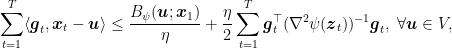
Lemma 2 For the two-steps OMD update above the following regret bound holds:
where
and
.
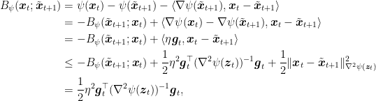
Proof: From the update rule, we have that
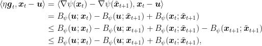
where in the second equality we used the 3-points equality for the Bregman divergences and the Generalized Pythagorean Theorem in the first inequality. Hence, summing over time we have

So, as we did in the previous lecture, we have
where
Putting all together, we have the stated bound.
This time it might be easier to get a handle over 


that is
Assuming 


Overall, we have the following improved regret guarantee for the Learning with Experts setting with positive losses.
Theorem 3 Assume
for
and
. Let
. Using OMD with the entropic regularizer
defined as
, learning rate
gives the following regret guarantee

Armed with this new tool, we can now turn to the multi-armed bandit problem again.
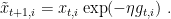
Let’s now consider the OMD with entropic regularizer, learning rate 

![\displaystyle \mathop{\mathbb E}\left[\sum_{t=1}^T g_{t,A_t}\right] - \sum_{t=1}^T \langle {\boldsymbol g}_t,{\boldsymbol u}\rangle = \mathop{\mathbb E}\left[\sum_{t=1}^T \langle \tilde{{\boldsymbol g}}_{t},{\boldsymbol x}_t\rangle - \sum_{t=1}^T \langle \tilde{{\boldsymbol g}}_t,{\boldsymbol u}\rangle\right] \leq \frac{B_\psi({\boldsymbol u}; {\boldsymbol x}_1)}{\eta} + \mathop{\mathbb E}\left[\sum_{t=1}^T \sum_{i=1}^d x_{t,i} \tilde{g}_{t,i}^2\right]~.](https://s0.wp.com/latex.php?latex=%5Cdisplaystyle+%5Cmathop%7B%5Cmathbb+E%7D%5Cleft%5B%5Csum_%7Bt%3D1%7D%5ET+g_%7Bt%2CA_t%7D%5Cright%5D+-+%5Csum_%7Bt%3D1%7D%5ET+%5Clangle+%7B%5Cboldsymbol+g%7D_t%2C%7B%5Cboldsymbol+u%7D%5Crangle+%3D+%5Cmathop%7B%5Cmathbb+E%7D%5Cleft%5B%5Csum_%7Bt%3D1%7D%5ET+%5Clangle+%5Ctilde%7B%7B%5Cboldsymbol+g%7D%7D_%7Bt%7D%2C%7B%5Cboldsymbol+x%7D_t%5Crangle+-+%5Csum_%7Bt%3D1%7D%5ET+%5Clangle+%5Ctilde%7B%7B%5Cboldsymbol+g%7D%7D_t%2C%7B%5Cboldsymbol+u%7D%5Crangle%5Cright%5D+%5Cleq+%5Cfrac%7BB_%5Cpsi%28%7B%5Cboldsymbol+u%7D%3B+%7B%5Cboldsymbol+x%7D_1%29%7D%7B%5Ceta%7D+%2B+%5Cmathop%7B%5Cmathbb+E%7D%5Cleft%5B%5Csum_%7Bt%3D1%7D%5ET+%5Csum_%7Bi%3D1%7D%5Ed+x_%7Bt%2Ci%7D+%5Ctilde%7Bg%7D_%7Bt%2Ci%7D%5E2%5Cright%5D%7E.+&bg=ffffff&fg=000000&s=0&c=20201002)
Now, focusing on the terms ![{\mathop{\mathbb E}[x_{t,i} \tilde{g}_{t,i}^2]}](https://s0.wp.com/latex.php?latex=%7B%5Cmathop%7B%5Cmathbb+E%7D%5Bx_%7Bt%2Ci%7D+%5Ctilde%7Bg%7D_%7Bt%2Ci%7D%5E2%5D%7D&bg=ffffff&fg=000000&s=0&c=20201002)
![\displaystyle \label{eq:expectation_exp3} \mathop{\mathbb E}\left[\sum_{i=1}^d x_{t,i} \tilde{g}_{t,i}^2\right] = \mathop{\mathbb E}\left[\mathop{\mathbb E}\left[\sum_{i=1}^d x_{t,i} \tilde{g}_{t,i}^2\middle|A_1, \dots, A_{t-1}\right]\right] = \mathop{\mathbb E}\left[\sum_{i=1}^d x_{t,i} \frac{g_{t,i}^2}{x_{t,i}}\right] \leq d L_\infty^2~. \ \ \ \ \ (2)](https://s0.wp.com/latex.php?latex=%5Cdisplaystyle+%5Clabel%7Beq%3Aexpectation_exp3%7D+%5Cmathop%7B%5Cmathbb+E%7D%5Cleft%5B%5Csum_%7Bi%3D1%7D%5Ed+x_%7Bt%2Ci%7D+%5Ctilde%7Bg%7D_%7Bt%2Ci%7D%5E2%5Cright%5D+%3D+%5Cmathop%7B%5Cmathbb+E%7D%5Cleft%5B%5Cmathop%7B%5Cmathbb+E%7D%5Cleft%5B%5Csum_%7Bi%3D1%7D%5Ed+x_%7Bt%2Ci%7D+%5Ctilde%7Bg%7D_%7Bt%2Ci%7D%5E2%5Cmiddle%7CA_1%2C+%5Cdots%2C+A_%7Bt-1%7D%5Cright%5D%5Cright%5D+%3D+%5Cmathop%7B%5Cmathbb+E%7D%5Cleft%5B%5Csum_%7Bi%3D1%7D%5Ed+x_%7Bt%2Ci%7D+%5Cfrac%7Bg_%7Bt%2Ci%7D%5E2%7D%7Bx_%7Bt%2Ci%7D%7D%5Cright%5D+%5Cleq+d+L_%5Cinfty%5E2%7E.+%5C+%5C+%5C+%5C+%5C+%282%29&bg=ffffff&fg=000000&s=0&c=20201002)
So, setting 
![\displaystyle \mathop{\mathbb E}\left[\sum_{t=1}^T g_{t,A_t}\right] - \sum_{t=1}^T \langle {\boldsymbol g}_t,{\boldsymbol u}\rangle \leq O\left(L_\infty \sqrt{d T \ln d}\right)~.](https://s0.wp.com/latex.php?latex=%5Cdisplaystyle+%5Cmathop%7B%5Cmathbb+E%7D%5Cleft%5B%5Csum_%7Bt%3D1%7D%5ET+g_%7Bt%2CA_t%7D%5Cright%5D+-+%5Csum_%7Bt%3D1%7D%5ET+%5Clangle+%7B%5Cboldsymbol+g%7D_t%2C%7B%5Cboldsymbol+u%7D%5Crangle+%5Cleq+O%5Cleft%28L_%5Cinfty+%5Csqrt%7Bd+T+%5Cln+d%7D%5Cright%29%7E.+&bg=ffffff&fg=000000&s=0&c=20201002)
Remark 2 The need for a different analysis for OMD is due to the fact that we want an easy way to upper bound the Hessian. Indeed, in this analysis
So, with a tighter analysis we showed that, even without an explicit exploration term, OMD with entropic regularizer solves the multi-armed bandit problem paying only a factor 
In the next section, we will see that changing the regularizer, with the same analysis, will remove the 
1. Optimal Regret Using OMD with Tsallis Entropy
In this section, we present the Implicitly Normalized Forecaster (INF) also known as OMD with Tsallis entropy for multi-armed bandit.
Define 
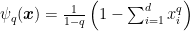
![{q \in [0,1]}](https://s0.wp.com/latex.php?latex=%7Bq+%5Cin+%5B0%2C1%5D%7D&bg=ffffff&fg=000000&s=0&c=20201002)


We will instantiate OMD with this regularizer for the multi-armed problem, as in Algorithm 2.

Note that 
We will not use any interpretation of this regularizer from the information theory point of view. As we will see in the following, the only reason to choose it is its Hessian. In fact, the Hessian of this regularizer is still diagonal and it is equal to

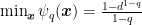
Now, we can use again the modified analysis for OMD in Lemma 2. So, for any 
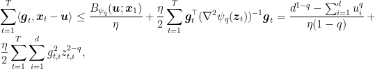
where
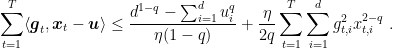
As we did for Exp3, now we need an upper bounds to the

that is

So, if
Hence, putting all together, we have
We can now specialize the above reasoning, considering 
Theorem 4 Assume
. Set
. Then, Algorithm 2
![\displaystyle \mathop{\mathbb E}\left[\sum_{t=1}^T g_{t,A_t}\right] - \sum_{t=1}^T \langle {\boldsymbol g}_t, {\boldsymbol u}\rangle \leq \frac{2\sqrt{d}}{\eta} + \eta \sqrt{d} L_\infty^2 T~.](https://s0.wp.com/latex.php?latex=%5Cdisplaystyle+%5Cmathop%7B%5Cmathbb+E%7D%5Cleft%5B%5Csum_%7Bt%3D1%7D%5ET+g_%7Bt%2CA_t%7D%5Cright%5D+-+%5Csum_%7Bt%3D1%7D%5ET+%5Clangle+%7B%5Cboldsymbol+g%7D_t%2C+%7B%5Cboldsymbol+u%7D%5Crangle+%5Cleq+%5Cfrac%7B2%5Csqrt%7Bd%7D%7D%7B%5Ceta%7D+%2B+%5Ceta+%5Csqrt%7Bd%7D+L_%5Cinfty%5E2+T%7E.+&bg=ffffff&fg=000000&s=0&c=20201002)
Proof: We only need to calculate the terms
![\displaystyle \mathop{\mathbb E}\left[\sum_{i=1}^d \tilde{g}^2_{t,i} x_{t,i}^{3/2}\right]~.](https://s0.wp.com/latex.php?latex=%5Cdisplaystyle+%5Cmathop%7B%5Cmathbb+E%7D%5Cleft%5B%5Csum_%7Bi%3D1%7D%5Ed+%5Ctilde%7Bg%7D%5E2_%7Bt%2Ci%7D+x_%7Bt%2Ci%7D%5E%7B3%2F2%7D%5Cright%5D%7E.+&bg=ffffff&fg=000000&s=0&c=20201002)
Proceeding as in (2), we obtain
![\displaystyle \begin{aligned} \mathop{\mathbb E}\left[\sum_{i=1}^d \tilde{g}^2_{t,i} x_{t,i}^{3/2}\right] &= \mathop{\mathbb E}\left[\mathop{\mathbb E}\left[\sum_{i=1}^d x_{t,i}^{3/2} \tilde{g}_{t,i}^2\middle|A_1, \dots, A_{t-1}\right]\right] = \mathop{\mathbb E}\left[\sum_{i=1}^d x_{t,i}^{3/2} \frac{g_{t,i}^2}{x_{t,i}^2} x_{t,i}\right] = \mathop{\mathbb E}\left[\sum_{i=1}^d g_{t,i}^2 \sqrt{x_{t,i}}\right] \\ &\leq \mathop{\mathbb E}\left[\sqrt{\sum_{i=1}^d g_{t,i}^2} \sqrt{\sum_{i=1}^d g_{t,i}^2 x_{t,i}}\right] \leq L_\infty \sqrt{d}~. \end{aligned}](https://s0.wp.com/latex.php?latex=%5Cdisplaystyle+%5Cbegin%7Baligned%7D+%5Cmathop%7B%5Cmathbb+E%7D%5Cleft%5B%5Csum_%7Bi%3D1%7D%5Ed+%5Ctilde%7Bg%7D%5E2_%7Bt%2Ci%7D+x_%7Bt%2Ci%7D%5E%7B3%2F2%7D%5Cright%5D+%26%3D+%5Cmathop%7B%5Cmathbb+E%7D%5Cleft%5B%5Cmathop%7B%5Cmathbb+E%7D%5Cleft%5B%5Csum_%7Bi%3D1%7D%5Ed+x_%7Bt%2Ci%7D%5E%7B3%2F2%7D+%5Ctilde%7Bg%7D_%7Bt%2Ci%7D%5E2%5Cmiddle%7CA_1%2C+%5Cdots%2C+A_%7Bt-1%7D%5Cright%5D%5Cright%5D+%3D+%5Cmathop%7B%5Cmathbb+E%7D%5Cleft%5B%5Csum_%7Bi%3D1%7D%5Ed+x_%7Bt%2Ci%7D%5E%7B3%2F2%7D+%5Cfrac%7Bg_%7Bt%2Ci%7D%5E2%7D%7Bx_%7Bt%2Ci%7D%5E2%7D+x_%7Bt%2Ci%7D%5Cright%5D+%3D+%5Cmathop%7B%5Cmathbb+E%7D%5Cleft%5B%5Csum_%7Bi%3D1%7D%5Ed+g_%7Bt%2Ci%7D%5E2+%5Csqrt%7Bx_%7Bt%2Ci%7D%7D%5Cright%5D+%5C%5C+%26%5Cleq+%5Cmathop%7B%5Cmathbb+E%7D%5Cleft%5B%5Csqrt%7B%5Csum_%7Bi%3D1%7D%5Ed+g_%7Bt%2Ci%7D%5E2%7D+%5Csqrt%7B%5Csum_%7Bi%3D1%7D%5Ed+g_%7Bt%2Ci%7D%5E2+x_%7Bt%2Ci%7D%7D%5Cright%5D+%5Cleq+L_%5Cinfty+%5Csqrt%7Bd%7D%7E.+%5Cend%7Baligned%7D&bg=ffffff&fg=000000&s=0&c=20201002)
Choosing 

There is one last thing, is how do we compute the prediction of this algorithm? In each step, we have to solve a constrained optimization problem. So, we can write the corresponding Lagragian:

From the KKT conditions, we have
![\displaystyle x_{t+1,i} = \left[\frac{1-q}{q}\left(\beta+ \frac{q}{1-q}x_{t,i}^{q-1}+\eta \tilde{g}_{t,i}\right)\right]^\frac{1}{q-1}~.](https://s0.wp.com/latex.php?latex=%5Cdisplaystyle+x_%7Bt%2B1%2Ci%7D+%3D+%5Cleft%5B%5Cfrac%7B1-q%7D%7Bq%7D%5Cleft%28%5Cbeta%2B+%5Cfrac%7Bq%7D%7B1-q%7Dx_%7Bt%2Ci%7D%5E%7Bq-1%7D%2B%5Ceta+%5Ctilde%7Bg%7D_%7Bt%2Ci%7D%5Cright%29%5Cright%5D%5E%5Cfrac%7B1%7D%7Bq-1%7D%7E.+&bg=ffffff&fg=000000&s=0&c=20201002)
and we also know that 

2. History Bits
The INF algorithm was proposed by (Audibert, J.-Y. and Bubeck, S., 2009) and re-casted as an OMD procedure in (Audibert, J.-Y. and Bubeck, S. and Lugosi, G., 2011). The connection with the Tsallis entropy was done in (Abernethy, J. D. and Lee, C. and Tewari, A., 2015). The specific proof presented here is new and it builds on the proof by (Abernethy, J. D. and Lee, C. and Tewari, A., 2015). Note that (Abernethy, J. D. and Lee, C. and Tewari, A., 2015) proved the same regret bound for a Follow-The-Regularized-Leader procedure over the stochastic estimates of the losses (that they call Gradient-Based Prediction Algorithm), while here we proved it using a OMD procedure.
3. Exercises
Exercise 1 Prove that in the modified proof of OMD, the terms
can be upper bounded by
.
Exercise 2 Building on the previous exercise, prove that regret bounds of the same order can be obtained for Exp3 and for the INF/OMD with Tsallis entropy directly upper bounding the terms

Hi Francesco, in the section of the Tsallis entropy, shouldn’t the Bregman divergence $ B_{\psi_q} (u, x_1) $ be equal to $ \frac{1}{1 – q} ( d^{1 – q} – \sum_{i=1}^d u_i^q ) $ (with the sum over $u_i^q$ instead of $\sqrt{x_i}$) ?
LikeLike
Fixed, thanks!
LikeLike
Sorry, shouldn’t it be $u_i$ instead of $x_i$? (which $x_i$ do you mean by the way?)
LikeLike
Right!! Fixed again.
LikeLike
Hi Francesco,
in Algorithm 2, line 7, shouldn’t it be x_{t+1} instead of tilde{x}_{t+1}?
LikeLike
Yes! Fixed, thanks
LikeLike