Implicit, Passive-Aggressive, and aProx updates

In this post, we talk about implicit updates in the online convex optimization framework (reminder: online ${\neq}$ stochastic). Instead, if you are interested in implicit updates in offline and stochastic optimization, I strongly suggest to read the amazing series of blogposts by Alex Shtof.

1. Implicit Updates

Let’s consider the two mostly commonly used frameworks for online learning: Online Mirror Descent (OMD) and Follow-The-Regularized-Leader (FTRL).

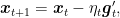
We already explained that in OMD we update the iterate as the minimizer of an linear approximation of the last loss function we received plus a term that measures the distance to the previous iterate:

$\displaystyle \begin{aligned} {\boldsymbol x}_{t+1} &= \mathop{\mathrm{argmin}}_{{\boldsymbol x} \in V} \ \ell_t({\boldsymbol x}_t) + \langle {\boldsymbol g}_t, {\boldsymbol x} - {\boldsymbol x}_t \rangle + \frac{1}{\eta_t}B_\psi({\boldsymbol x};{\boldsymbol x}_{t}) \\ &= \mathop{\mathrm{argmin}}_{{\boldsymbol x} \in V} \ \langle {\boldsymbol g}_t, {\boldsymbol x} \rangle + \frac{1}{\eta_t}B_\psi({\boldsymbol x};{\boldsymbol x}_{t}), \end{aligned}$

where ${{\boldsymbol g}_t \in \partial \ell_t({\boldsymbol x}_t)}$ .

On the other hand, in FTRL we have two possibilities: we can minimize the regularized sum of the loss we have received till now or the regularized sum of the linear approximation of the losses. In the first case, we update with

$\displaystyle {\boldsymbol x}_{t+1} = \mathop{\mathrm{argmin}}_{{\boldsymbol x} \in V} \ \psi_{t+1} ({\boldsymbol x})+ \sum_{i=1}^t \ell_i({\boldsymbol x}),$

while in the second case, we use

$\displaystyle \begin{aligned} {\boldsymbol x}_{t+1} &= \mathop{\mathrm{argmin}}_{{\boldsymbol x} \in V} \ \psi_{t+1} ({\boldsymbol x}) + \sum_{i=1}^t \left(\ell_i({\boldsymbol x}_i) +\langle {\boldsymbol g}_i, {\boldsymbol x}-{\boldsymbol x}_i\rangle\right)\\ &= \mathop{\mathrm{argmin}}_{{\boldsymbol x} \in V} \ \psi_{t+1} ({\boldsymbol x}) + \sum_{i=1}^t \langle {\boldsymbol g}_i, {\boldsymbol x}\rangle, \end{aligned}$

where ${{\boldsymbol g}_i \in \partial \ell_i({\boldsymbol x}_i)}$ for ${i=1, \dots, t}$ . The second update is what optimization people call Dual Averaging. We also saw that under some reasonable conditions, the two updates of FTRL have the same regret guarantee. However, we would expect the second approach, the one using the exact loss functions, to perform much better in practice. Also, in the linearization of the losses we have to assume to know some characteristics of the losses, e.g., strong convexity parameter, to achieve the same regret of the full-losses FTRL.

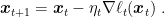
Overall, we have two different frameworks and two different ways to use the loss functions in the update. So, it should be obvious that there is at least another possibility, that is OMD with exact loss. That is, we would like to consider the update

$\displaystyle \label{eq:omd_implicit} {\boldsymbol x}_{t+1} = \mathop{\mathrm{argmin}}_{{\boldsymbol x} \in V} \ \ell_t({\boldsymbol x}) + \frac{1}{\eta_t}B_\psi({\boldsymbol x};{\boldsymbol x}_{t})~. \ \ \ \ \ (1)$

As in the FTRL case, we would expect this update to be better than the linearized one, at least empirically.

To gain some more intuition, let’s consider the simple case that ${\psi({\boldsymbol x}) =\frac{1}{2} \|{\boldsymbol x}\|_2^2}$ , ${V={\mathbb R}^d}$ , and the losses ${\ell}$ are differentiable. In this case, we have that the linearized OMD update becomes

$\displaystyle {\boldsymbol x}_{t+1} = {\boldsymbol x}_t - \eta_t \nabla \ell_t({\boldsymbol x}_t)~.$

For example, with square loss and linear predictors over couples input/labels ${({\boldsymbol z}_t,y_t)}$ , we have ${\ell_t({\boldsymbol x}) = \frac{1}{2} (\langle {\boldsymbol z}_t, {\boldsymbol x}\rangle - y_t)^2}$ and the update becomes

$\displaystyle {\boldsymbol x}_{t+1} = {\boldsymbol x}_t - \eta_t {\boldsymbol z}_t (\langle {\boldsymbol z}_t, {\boldsymbol x}_t\rangle - y_t)~.$

On the other hand, the update of OMD with the exact loss function becomes

$\displaystyle \label{eq:implicit_ogd} {\boldsymbol x}_{t+1} = \mathop{\mathrm{argmin}}_{{\boldsymbol x}} \ \ell_t({\boldsymbol x}) + \frac{1}{2\eta_t} \|{\boldsymbol x} - {\boldsymbol x}_t\|^2_2~. \ \ \ \ \ (2)$

The optimality condition tells us that ${{\boldsymbol x}_{t+1}}$ satisfies

$\displaystyle \nabla \ell_t ({\boldsymbol x}_{t+1}) + \frac{1}{\eta_t} ({\boldsymbol x}_{t+1} - {\boldsymbol x}_t) = \boldsymbol{0},$

that is

$\displaystyle {\boldsymbol x}_{t+1} = {\boldsymbol x}_t - \eta_t \nabla \ell_t ({\boldsymbol x}_{t+1})~.$

So, the update is not in a closed formula anymore, but it has an implicit form, where ${{\boldsymbol x}_{t+1}}$ appears in both side of the equality. This is exactly the reason why the update of OMD with exact losses is known in the online learning literature as implicit updates. So, we will call the update in (1) Implicit OMD.

Remark 1. Observe that for linear losses OMD and the Implicit OMD are equivalent.

In general, calculating the update of Implicit OMD can be an annoying optimization problem. However, in some cases the Implicit OMD update can still be solved in a closed form.

Example 1. Consider again linear regression with square loss. The update of Implicit OMD becomes

$\displaystyle \label{eq:upd_impl_sq} {\boldsymbol x}_{t+1} = {\boldsymbol x}_t - \eta_t {\boldsymbol z}_t (\langle {\boldsymbol z}_t, {\boldsymbol x}_{t+1}\rangle - y_t)~. \ \ \ \ \ (3)$

To solve the equation, we take the inner product of both sides with ${{\boldsymbol z}_t}$ , to obtain

$\displaystyle \langle {\boldsymbol z}_t,{\boldsymbol x}_{t+1} \rangle = \langle {\boldsymbol z}_t, {\boldsymbol x}_t \rangle - \eta_t \|{\boldsymbol z}_t\|^2_2 (\langle {\boldsymbol z}_t, {\boldsymbol x}_{t+1}\rangle - y_t)$

that is

$\displaystyle \langle {\boldsymbol z}_t,{\boldsymbol x}_{t+1} \rangle = \frac{\langle {\boldsymbol z}_t, {\boldsymbol x}_t \rangle + \eta_t \|{\boldsymbol z}_t\|^2_2 y_t}{1+ \eta_t \|{\boldsymbol z}_t\|^2_2}~.$

Substituting this expression in (3), we have

$\displaystyle {\boldsymbol x}_{t+1} = {\boldsymbol x}_t - \eta_t {\boldsymbol z}_t \left(\frac{\langle {\boldsymbol z}_t, {\boldsymbol x}_t \rangle + \eta_t \|{\boldsymbol z}_t\|^2_2 y_t}{1+ \eta_t \|{\boldsymbol z}_t\|^2_2}- y_t\right) = {\boldsymbol x}_t - \frac{\eta_t}{1 + \eta_t \|{\boldsymbol z}_t\|^2_2} {\boldsymbol z}_t (\langle {\boldsymbol z}_t, {\boldsymbol x}_{t}\rangle - y_t)~.$

Implicit Updates are Always Descending Till now, we have motivated implicit updates purely from an intuitive point of view: We expect this algorithm to be better because we do not approximate the loss functions. Indeed, we often gain a lot in performance switching to implicit updates. However, we can even prove that implicit updates have interesting theoretical properties.

First, contrarily to OGD, implicit updates remains “sane” even when the learning rate goes to infinity. Indeed, taking ${\eta_t}$ to infinity in (1), ${{\boldsymbol x}_{t+1}}$ becomes simply the minimizer of the loss function. On the other hand, in OMD when the learning rate goes to infinity we can take a step that is arbitrarily far from the minimizer of the function!

When we consider non-differentiable convex functions, there is another important difference between implicit updates and subgradient descent updates. We already saw that the subgradient might not point in a descent direction. That is, no matter how we choose ${\eta_t>0}$ , the value of the function in ${{\boldsymbol x}_{t+1}}$ might be higher than in ${{\boldsymbol x}_{t}}$ . On the other hand, this cannot happen with implicit updates, no matter how we choose the learning rate:

$\displaystyle \begin{aligned} \ell({\boldsymbol x}_{t+1}) &< \ell({\boldsymbol x}_{t+1}) + \frac{1}{\eta_t} B_\psi({\boldsymbol x}_{t+1};{\boldsymbol x}_{t}) = \mathop{\mathrm{argmin}}_{{\boldsymbol x} \in V} \ \ell({\boldsymbol x}) + \frac{1}{\eta_t} B_\psi({\boldsymbol x};{\boldsymbol x}_{t}) \\ &\leq \ell({\boldsymbol x}_t) + \frac{1}{\eta_t} B_\psi({\boldsymbol x}_{t};{\boldsymbol x}_{t}) = \ell({\boldsymbol x}_t)~. \end{aligned}$

Proximal updates Are implicit updates actually an invention of online learning people? Actually, no. Indeed, these kind of updates were known at least in 1965 (!) and they were proposed for the (offline) optimization of functions with the name of proximal updates. Basically, we have a function ${\ell({\boldsymbol x})}$ and we minimize it iteratively with the update

$\displaystyle \label{eq:prox_upd} {\boldsymbol x}_{t+1} = \mathop{\mathrm{argmin}}_{{\boldsymbol x}} \ \ell({\boldsymbol x}) + \frac{1}{2\eta_t} \|{\boldsymbol x} - {\boldsymbol x}_{t+1}\|^2_2, \ \ \ \ \ (4)$

starting from an initial point ${{\boldsymbol x}_1 \in \mathop{\mathrm{dom}} \ell}$ . At first sight, such update might seem pointless in offline optimization: being able to solve (4) implies being also able to find the minimizer of ${\ell}$ in one step! However, as we have previously discussed, these kind of updates find an application when the function ${\ell}$ is composed by two parts and we decide to linearize only one part.

2. Passive-Aggressive

Now, let me show you that implicit updates were actually used a lot in the online literature, even if many people did not realize it.

Let’s take a look at a very famous online learning algorithm: the Passive-Aggressive (PA) algorithm. PA was a major success in online learning: 2099 citations and counting, that is huge for the online learning area. The theory was not very strong, but the performance of these algorithms was way better than anything else we had at that time. Let’s see how the PA algorithm works.

The PA algorithm was introduced before the Online Convex Optimization (OCO) framework was proposed. So, at that time, online learning for classification and regression focused on the particular case in which the loss functions have the form ${\ell_t({\boldsymbol x}) = \ell( \langle {\boldsymbol x}, {\boldsymbol z}_t\rangle, {\boldsymbol y}_t)}$ , basically the loss of linear predictors over couples input/label ${({\boldsymbol z}_t,y_t)}$ . The PA algorithm in particular focused on losses that can be zero over intervals, like the hinge loss, the squared hinge loss, the ${\epsilon}$ -insensitive loss, and the squared ${\epsilon}$ -insensitive loss. For these losses, the update they proposed was

$\displaystyle {\boldsymbol x}_{t+1} = \mathop{\mathrm{argmin}}_{{\boldsymbol x}} \ C \ell_t({\boldsymbol x}) + \frac{1}{2} \|{\boldsymbol x} - {\boldsymbol x}_t\|^2_2,$

where ${C>0}$ is a hyperparameter. Now, this is exactly the Implicit OMD update with the special case of the squared L2 Bregman divergence! The choice of the loss functions makes this update always in a closed form. So, for example, for the hinge loss and linear predictors, we have

$\displaystyle \label{eq:pa_update} {\boldsymbol x}_{t+1} = \mathop{\mathrm{argmin}}_{{\boldsymbol x}} \ C \max(1-y_t\langle {\boldsymbol x}, {\boldsymbol z}_t\rangle,0) + \frac{1}{2} \|{\boldsymbol x} - {\boldsymbol x}_t\|^2_2 = {\boldsymbol x}_t - \min\left(C,\frac{\max(1-y_t\langle {\boldsymbol x}_t, {\boldsymbol z}_t\rangle,0)}{\|{\boldsymbol z}_t\|^2_2}\right) y_t {\boldsymbol z}_t, \ \ \ \ \ (5)$

where the second equality is calculated using the optimality condition and it is left as an exercise to the reader.

So, the huge boost in performance of PA over other online algorithm is due uniquely to the implicit updates.

3. Implicit Updates on Truncated Linear Models: aProx

There is another first-order optimization algorithm inspired to implicit updates. As we said, implicit updates are rarely in a closed form. So, we can try to approximate the implicit updates in some way. One possibility is to use the implicit update on a surrogate loss function. Indeed, when we use a linear approximation we recover plain OMD. Instead, when we use the exact function we get the implicit updates. What can we use in between the two cases? We could think to use a truncated linear model. That is, in the case we know that the functions are lower bounded by some ${\ell_\text{low}>-\infty}$ , we define

$\displaystyle \tilde{\ell}_t({\boldsymbol u}; {\boldsymbol x}_t) := \max(\ell_t({\boldsymbol x}_t) + \langle {\boldsymbol g}_t, {\boldsymbol u}-{\boldsymbol x}_t\rangle, \ell_\text{low}),$

for any ${{\boldsymbol g}_t \in \partial \ell_t({\boldsymbol x}_t)}$ . Note that this is a lower bound to the loss function ${\ell_t}$ and it is piecewise linear.

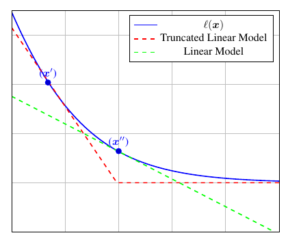
truncated_linear_model — Truncated linear model (Red) built around the point ${{\boldsymbol x}}$ , and a linear model (Green) built around the point ${{\boldsymbol x}''}$ .

Now, we can use these surrogate function in the implicit OMD:

$\displaystyle {\boldsymbol x}_{t+1} = \mathop{\mathrm{argmin}}_{{\boldsymbol x} \in V} \ \tilde{\ell}_t({\boldsymbol x};{\boldsymbol x}_t) + \frac{1}{\eta_t}B_\psi({\boldsymbol x};{\boldsymbol x}_{t})~.$

Implicit OMD with truncated linear models and the squared L2 Bregman is called aProx (Asi and Duchi, 2019).

Considering ${V={\mathbb R}^d}$ and ${\psi({\boldsymbol x})=\frac12 \|{\boldsymbol x}\|^2_2}$ , we again have

$\displaystyle {\boldsymbol x}_{t+1} = {\boldsymbol x}_t - \eta_t {\boldsymbol g}'_t,$

where ${{\boldsymbol g}'_t}$ is a specific vector in ${\partial \tilde{\ell}_t({\boldsymbol x}_{t+1};{\boldsymbol x}_t)}$ . Now, we have 2 possibilities: ${{\boldsymbol x}_{t+1}}$ is in the flat part or in the corner of ${\tilde{\ell}_t}$ . Indeed, it should be easy to see that the proximal update assures us that we cannot miss the corner and land on the flat part. So, if we are in the linear part, then ${{\boldsymbol g}'_t={\boldsymbol g}_t}$ . Instead, if we are in the corner we have ${{\boldsymbol g}'_t = \alpha_t {\boldsymbol g}_t }$ where ${\alpha_t \in [0,1]}$ . Hence, we always have

$\displaystyle {\boldsymbol x}_{t+1} = {\boldsymbol x}_t - \eta_t \alpha_t {\boldsymbol g}_t$

and we only need to find ${\alpha_t}$ . Substituting ${{\boldsymbol x}_{t+1}}$ in the definition of ${\tilde{\ell}_t}$ and using first-order optimality condition, we can verify that the following is the closed formula of the update (left as an exercise)

$\displaystyle {\boldsymbol x}_{t+1} = {\boldsymbol x}_t - {\boldsymbol g}_t \min\left(\eta_t, \frac{\ell_t({\boldsymbol x}_t)- \ell_\text{low}}{\|{\boldsymbol g}_t\|^2}\right)~.$

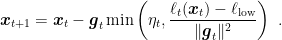
The similarity between this update and the one of PA in (5) should be adamant, that is due to the similarity between the truncated linear model and the hinge loss. Indeed, running aProx on linear classifiers with hinge loss is exactly the PA algorithm.

4. More Updates Similar to the Implicit Updates

From an empirical point of view, we can gain a lot of performance using implicit updates, even just approximating them. So, it should not be surprising if people proposed and used similar ideas in many optimization algorithm. Let me give you some examples.

The default optimization algorithm in the machine learning library Vowpal Wabbit (VW) uses the Importance Weight Aware Updates (Karampatziakis and Langford, 2011). These updates essentially approximate the implicit update using a differential equation that for linear models can be calculated in a closed formula. So, if you ever used VW, you already used a close relative of implicit updates, probably without knowing it.

Another interesting example is the setting of adaptive filtering, where one wants to minimize ${\sum_{t=1}^T (\langle {\boldsymbol z}_t, {\boldsymbol x}_t\rangle-\langle {\boldsymbol z}_t,{\boldsymbol u}\rangle)^2}$ . In this setting, a classic algorithm is Least Mean Squared (LMS) algorithm that corresponds to Online Gradient Descent with linear models and squared loss. Now, a known better version of the LMS is the normalized LMS, that is nothing else that Implicit OMD with linear models and squared loss.

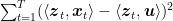
There are even interpretations of the Nesterov’s accelerated gradient method as an implicit update on a curved space (Defazio, 2019).

So, implicit updates are so “natural” that I personally think that any offline/online optimization algorithm that has good performance must be a good approximation of implict updates. Hence, I am sure there are even more examples of implicit updates hiding in other well-known algorithms.

5. Regret Guarantee for Implicit Updates

From the above reasoning, it seems very intuitive to expect a better regret bound for implicit updates. However, it turns out particularly challenging to prove a quantifiable advantage of implicit updates over OMD ones in the adversarial setting.

Here, I show a very recent result of mine on Implicit OMD that for the first time shows a clear advantage of Implicit OMD in some situations.

First, we can show the following theorem.

Theorem 1. Assume a constant learning rate ${\eta_t=\eta>0}$ . Then, implicit OMD guarantees

$\displaystyle \sum_{t=1}^T \ell_t({\boldsymbol x}_t) - \sum_{t=1}^T \ell_t({\boldsymbol u}) \leq \frac{B_\psi({\boldsymbol u}; {\boldsymbol x}_1)}{\eta} + \sum_{t=1}^T \left( \ell_t({\boldsymbol x}_t) - \ell_t({\boldsymbol x}_{t+1}) -\frac{1}{\eta}B_\psi({\boldsymbol x}_{t+1}; {\boldsymbol x}_t)\right), \forall {\boldsymbol u} \in V,$

Moreover, assume the distance generating function to be 1-strongly convex w.r.t. ${\|\cdot\|}$ . Then, there exists ${{\boldsymbol g}_t' \in \partial \ell_t({\boldsymbol x}_{t+1})}$ such that we have

$\displaystyle \ell_t({\boldsymbol x}_t) - \ell_t({\boldsymbol x}_{t+1}) -\frac{1}{\eta}B_\psi({\boldsymbol x}_{t+1}; {\boldsymbol x}_t) \leq \min\left( \frac{\eta}{2} \|{\boldsymbol g}_t\|^2, 2 \eta \|{\boldsymbol g}_t\|_\star \|{\boldsymbol g}_t'\|_\star\right), \ \forall {\boldsymbol g}_t \in \partial \ell_t({\boldsymbol x}_t)~.$

Proof: To obtain this bound, we proceed in a slightly different way than in the classic OMD proof. In particular, for any ${{\boldsymbol u} \in V}$ we have

$\displaystyle \begin{aligned} \eta (\ell_t({\boldsymbol x}_{t+1}) - \ell_t({\boldsymbol u})) & \leq \langle \eta {\boldsymbol g}_t', {\boldsymbol x}_{t+1} - {\boldsymbol u} \rangle \leq \langle \nabla \psi({\boldsymbol x}_t) - \nabla \psi({\boldsymbol x}_{t+1}), {\boldsymbol x}_{t+1} - {\boldsymbol u} \rangle \\ & = B_\psi ({\boldsymbol u}; {\boldsymbol x}_t ) - B_\psi({\boldsymbol u}; {\boldsymbol x}_{t+1}) - B_\psi({\boldsymbol x}_{t+1}; {\boldsymbol x}_t ), \end{aligned}$

where ${{\boldsymbol g}_t' \in \partial \ell_t({\boldsymbol x}_{t+1})}$ and in the second inequality we have used the optimality condition of the update. Adding ${\eta \ell_t({\boldsymbol x}_t)}$ to both terms of the inequality, dividing by ${\eta}$ , and reordering, we have

$\displaystyle \ell_t({\boldsymbol x}_t) - \ell_t({\boldsymbol u}) \leq \frac{1}{\eta} \left( B_\psi ({\boldsymbol u}; {\boldsymbol x}_t ) - B_\psi({\boldsymbol u}; {\boldsymbol x}_{t+1}) - B_\psi({\boldsymbol x}_{t+1}; {\boldsymbol x}_t ) \right)+ \ell_t({\boldsymbol x}_t) - \ell_t({\boldsymbol x}_{t+1}) ~.$

Summing over time, we get the first bound.

For the second bound, let’s now focus on the terms ${- \frac{1}{\eta}B_\psi({\boldsymbol x}_{t+1}; {\boldsymbol x}_t ) + \ell_t({\boldsymbol x}_t) - \ell_t({\boldsymbol x}_{t+1})}$ and we upper bound them in two different ways. First, using the convexity of the losses, we can bound the difference between ${\ell_t({\boldsymbol x}_t)}$ and ${\ell_t({\boldsymbol x}_{t+1})}$ :

$\displaystyle \ell_t({\boldsymbol x}_t) - \ell_t ({\boldsymbol x}_{t+1}) \leq \langle {\boldsymbol g}_t, {\boldsymbol x}_t - {\boldsymbol x}_{t+1} \rangle \leq \| {\boldsymbol g}_t \|_\star \| {\boldsymbol x}_t - {\boldsymbol x}_{t+1} \|,$

where ${{\boldsymbol g}_t \in \partial \ell_t({\boldsymbol x}_t)}$ . Also, from the strong convexity of ${\Psi}$ , we have

$\displaystyle \frac{1}{2} \|{\boldsymbol x}_{t+1} - {\boldsymbol x}_t\|^2 \leq B_\psi({\boldsymbol x}_{t+1}; {\boldsymbol x}_t) ~.$

Hence, putting all together we have

$\displaystyle - \frac{1}{\eta}B_\psi({\boldsymbol x}_{t+1}; {\boldsymbol x}_t ) + \ell_t({\boldsymbol x}_t) - \ell_t({\boldsymbol x}_{t+1}) \leq \| {\boldsymbol g}_t \|_\star \| {\boldsymbol x}_t - {\boldsymbol x}_{t+1} \| - \frac{1}{2\eta} \|{\boldsymbol x}_{t+1} - {\boldsymbol x}_t\|^2 \leq \frac{\eta}{2}\|{\boldsymbol g}_t\|^2_\star,$

where in the last inequality we used the elementary inequality ${bx - \frac{a}{2} x^2 \leq \frac{b^2}{2 a}, \forall x \in {\mathbb R}}$ .

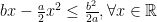
From the optimality condition of the implicit OMD update, we know that there exists ${{\boldsymbol g}_t'\in \partial \ell_t({\boldsymbol x}_{t+1})}$ such that

$\displaystyle \langle \eta {\boldsymbol g}_t' + \nabla \psi({\boldsymbol x}_{t+1}) -\nabla \psi({\boldsymbol x}_t), {\boldsymbol u}-{\boldsymbol x}_{t+1}\rangle \geq 0, \ \forall {\boldsymbol u} \in V~.$

Hence, we have

$\displaystyle \begin{aligned} \frac{1}{2} \|{\boldsymbol x}_{t+1} - {\boldsymbol x}_t\|^2 &\leq B_\psi({\boldsymbol x}_{t+1}; {\boldsymbol x}_t) \leq \langle \nabla \psi({\boldsymbol x}_{t+1}) - \nabla \psi({\boldsymbol x}_t), {\boldsymbol x}_{t+1} - {\boldsymbol x}_t \rangle \leq \langle \eta {\boldsymbol g}'_t, {\boldsymbol x}_t - {\boldsymbol x}_{t+1}\rangle \\ &\leq \eta \|{\boldsymbol g}'_t\|_\star \, \|{\boldsymbol x}_{t+1} - {\boldsymbol x}_t \|, \end{aligned}$

where we used the convexity of the Bregman divergence in its first argument in the second inequality and the optimality condition of the update in the third inequality. This chain of inequalities implies that ${ \|{\boldsymbol x}_{t+1} - {\boldsymbol x}_t\|\leq 2 \eta \|{\boldsymbol g}'_t\|_\star}$ that gives the second bound in the minimum. $\Box$

The theorem shows a possible and small improvement over the OMD regret bound. In particular, there might be sequences of losses where ${4 \|{\boldsymbol g}'_{t+1}\|_\star < \|{\boldsymbol g}_t\|_\star}$ . The fact that the improvement is only possible on some sequences is to be expected: the OMD regret is worst-case optimal on bounded domains, so there is not much to gain. However, maybe we could expect a larger gain on some particular sequence of functions. Indeed, we can show that on some sequences of losses we can achieve constant regret! Let’s see how.

From the regret above, we have

$\displaystyle \begin{aligned} \sum_{t=1}^T \ell_t({\boldsymbol x}_t) - \sum_{t=1}^T \ell_t({\boldsymbol u}) &\leq \frac{B_\psi({\boldsymbol u}, {\boldsymbol x}_1)}{\eta} + \sum_{t=1}^T \left(\ell_t({\boldsymbol x}_t) - \ell_t({\boldsymbol x}_{t+1}) - \frac{B_\psi({\boldsymbol x}_{t+1}, {\boldsymbol x}_t)}{\eta} \right)\\ &\leq \frac{B_\psi({\boldsymbol u}, {\boldsymbol x}_1)}{\eta} + \ell_1({\boldsymbol x}_1) - \ell_T({\boldsymbol x}_{T+1}) + \sum_{t=2}^T \left( \max_{{\boldsymbol x} \in V} \ \ell_t({\boldsymbol x}) - \ell_{t-1}({\boldsymbol x}) \right) ~. \end{aligned}$

Denoting by ${V_T:=\sum_{t=2}^T \left( \max_{{\boldsymbol x} \in V} \ \ell_t({\boldsymbol x}) - \ell_{t-1}({\boldsymbol x}) \right)}$ the temporal variability of the losses, we have that the regret guarantee is

$\displaystyle \sum_{t=1}^T \ell_t({\boldsymbol x}_t) - \sum_{t=1}^T \ell_t({\boldsymbol u}) \leq \frac{B_\psi({\boldsymbol u}, {\boldsymbol x}_1)}{\eta} + \ell_1({\boldsymbol x}_1) - \ell_T({\boldsymbol x}_{T+1}) + V_T~.$

Now, in the case that the loss functions are all the same ${V_T=0}$ and the regret upper bound becomes a constant independent of ${T}$ . It is worth reminding that constant regret is the best we can hope for in online convex optimization! In other words, when online learning becomes as easy as offline learning (i.e., all the losses are equal), that implicit updates give us a provable large boost.

However, there is a caveat: In order to get a ${\sqrt{T}}$ regret in the general case we need ${\eta\propto \frac{1}{\sqrt{T}}}$ . On the other had, if ${V_T=O(1)}$ we want ${\eta=O(1)}$ . The problem in online learning learning is that we do not know the future, so we need some adaptive strategy that changes ${\eta_t}$ in a dynamic way. This is indeed possible and we leave this as an exercise, see below.

Our last observation is that we can recover the constant regret bound even for FTRL when used on the exact losses. Again, this is due to the use of the exact losses rather than the linear approximation. Remember that FTRL predicts with ${{\boldsymbol x}_t \in \mathop{\mathrm{argmin}}_{{\boldsymbol x} \in V} \ F_{t}({\boldsymbol x})}$ , where ${F_t({\boldsymbol x}) = \psi_{t}({\boldsymbol x}) + \sum_{i=1}^{t-1} \ell_i({\boldsymbol x})}$ . Hence, from the FTRL regret equality and assuming a non-decreasing regularizer, we have

$\displaystyle \begin{aligned} \sum_{t=1}^T ( \ell_t({\boldsymbol x}_t) - \ell_t({\boldsymbol u}) ) &= \psi_{T+1}({\boldsymbol u}) - \min_{{\boldsymbol x} \in V} \ \psi_{1}({\boldsymbol x}) + \sum_{t=1}^T [F_t({\boldsymbol x}_t) - F_{t+1}({\boldsymbol x}_{t+1}) + \ell_t({\boldsymbol x}_t)] + F_{T+1}({\boldsymbol x}_{T+1}) - F_{T+1}({\boldsymbol u}) \\ &\leq \psi_{T+1}({\boldsymbol u}) - \min_{{\boldsymbol x} \in V} \ \psi_{1}({\boldsymbol x}) + \sum_{t=1}^T (\ell_t({\boldsymbol x}_{t}) - \ell_t({\boldsymbol x}_{t+1}))\\ &\leq \psi_{T+1}({\boldsymbol u}) - \min_{{\boldsymbol x} \in V} \ \psi_{1}({\boldsymbol x}) + \ell_1({\boldsymbol x}_1) - \ell_T({\boldsymbol x}_{T+1}) + \sum_{t=2}^T \left( \max_{{\boldsymbol x} \in V} \ \ell_t({\boldsymbol x}) - \ell_{t-1}({\boldsymbol x}) \right) \\ &= \psi_{T+1}({\boldsymbol u}) - \min_{{\boldsymbol x} \in V} \ \psi_{1}({\boldsymbol x}) + \ell_1({\boldsymbol x}_1) - \ell_T({\boldsymbol x}_{T+1}) + V_T~. \end{aligned}$

However, FTRL with exact losses requires to solve a finite sum optimization problem whose size grows with the number of iterations. Instead, Implicit OMD uses only one loss in each round, resulting in a closed formula in a number of interesting cases. We also note that we would have the same tuning problem as before: in order to get a constant regret when ${V_T=O(1)}$ , we would need the regularizer to be constant and independent from time, while it should grow as ${\sqrt{T}}$ in the general case.

6. History Bits

The implicit updates in online learning were proposed for the first time by (Kivinen and Warmuth, 1997). However, such update with the Euclidean divergence is the Proximal update in the optimization literature dating back at least to 1965 (Moreau, 1965)(Martinet, 1970)(Rockafellar, 1976)(Parikh and Boyd, 2014), and more recently used even in the stochastic setting (Toulis and Airoldi, 2017)(Asi and Duchi, 2019).

The PA algorithms were proposed in (Crammer et al., 2006), but the connection with implicit updates was absent in the paper. I am not sure who first realized the connection: I realized it in 2011 and I showed it to Joseph Keshet (one of the author of PA) that encouraged me to publish it somewhere. Only 10 years later, I am doing it 🙂 Note that the mistake bound proved in the PA paper is worse than the Perceptron bound. Later, we proved a mistake bound for PA that is strictly better than the classic Perceptron’s bound (Jie et al., 2010).

The very nice idea of truncated linear models was proposed by (Asi and Duchi, 2019) as a way to approximate proximal updates and retaining closed form updates.

The connection between implicit OMD and normalized LMS was shown by (Kivinen et al., 2006).

(Kulis and Bartlett, 2010) provide the first regret bounds for implicit updates that match those of OMD, while (McMahan, 2010) makes the first attempt to quantify the advantage of the implicit updates in the regret bound. Finally, (Song et al., 2018) generalize the results in (McMahan, 2010) to Bregman divergences and strongly convex functions, and quantify the gain differently in the regret bound. Note that in (McMahan, 2010)(Song et al., 2018) the gain cannot be exactly quantified, providing just a non-negative data-dependent quantity subtracted to the regret bound. The connection between temporal variation and implicit updates was shown in (Campolongo and Orabona, 2020), together with a matching lower bound.

7. Acknowledgements

Thanks to Nicolò Campolongo for feedback on a draft of this post.

8. Exercises

Exercise 1. Prove that the update of PA given above is correct.

Exercise 2. Prove that the update of aProx given above is correct.

Exercise 3. Find an learning rate strategy to adapt to the value of ${V_T}$ without knowing it (Campolongo and Orabona, 2020).

2 Comments

Pedro Zattoni Scroccaro says:

February 15, 2022 at 5:01 AM

Is the \eta/2 multiplying the first inequality of Theorem 1 a typo?

LikeLiked by 1 person

1. bremen79 says:
  
  February 15, 2022 at 3:48 PM
  
  You are right! Fixed, thanks.
  
  LikeLike

Parameter-free Learning and Optimization Algorithms

Implicit, Passive-Aggressive, and aProx updates

2 Comments

Leave a Reply Cancel reply

Share this:

Like this:

Related

Leave a Reply Cancel reply