The Weighted Average Algorithm

This time we will introduce the Weighted Average Algorithm (WAA). I will do it my way: I am allergic to present for each algorithm a different analysis! From my blog it should be clear that we only have two main algorithms in online learning: OMD and FTRL. So, 99% of the online algorithms are instantiations of one or the other. In this case, I will show that WAA is nothing else than FTRL on distributions.

Next time, I will introduce the Aggregating Algorithm (AA) as a variant of the WAA.

1. Follow-the-Regularized-Leader with Distributions

Our analysis of the WAA will be based on a generalization of the FTRL algorithm with the entropic regularizer, to work with distributions with infinite support, either countable or continuous.

Let ${\mathcal{X} \subseteq {\mathbb R}^d}$ the intersection of all domains of ${\ell_t}$ , ${m}$ be a fixed measure on ${\mathcal{X}}$ , and ${P_1}$ be some probability density with respect to ${m}$ (this means that ${\int_\mathcal{X} P_1({\boldsymbol x}) m(\mathrm{d} {\boldsymbol x}) =1}$ ; in what follows, we will drop “with respect to ${m}$ ”). In the finite case, it is natural to take ${m(i)=1, i=1, \dots, k}$ (the counting measure), while in the continuous case the natural choice of ${m}$ is the Lebesgue measure.

For some set of distributions ${\mathcal{P}}$ , in each round we output ${P_t \in \mathcal{P}}$ , then we receive the loss functions ${f_t(P):=\mathop{\mathbb E}_{{\boldsymbol x} \sim P}[\ell_t({\boldsymbol x})]}$ , where ${\ell_t:\mathcal{X} \rightarrow {\mathbb R}}$ . To simplify the notation, we introduce the duality pairing

$\displaystyle \langle \ell, P \rangle := \int \!\ell({\boldsymbol x}) P(\mathrm{d} {\boldsymbol x})~.$

Note that the duality pairing is bi-linear but not symmetric, so it should not be confused with the inner product. Yet, it reduces to the inner product in some cases, for example, when ${\mathcal{V}}$ is a discrete set. With this notation, we can write ${f_t(P)=\langle \ell_t, P\rangle}$ . We also have that the functional derivative of ${f_t}$ is

$\displaystyle \nabla_P f_t=\ell_t~.$

The above notation will greatly facilitate the generalization of FTRL to infinite distributions. Let’s use FTRL with regularizers ${\psi_t:\mathcal{P}\rightarrow {\mathbb R}}$ . Hence, at round ${t}$ we produce a probability distribution ${P_t}$ defined as

$\displaystyle \mathop{\mathrm{argmin}}_{P \in \mathcal{P}} \ \left(F_t(P):=\psi_t(P) + \left\langle\sum_{i=1}^{t-1} \ell_i,P\right\rangle\right)~.$

It is easy to see that the FTRL equality works even in this setting, so we have that

$\displaystyle \left\langle\sum_{t=1}^T - \ell_t,Q\right\rangle = \psi_{T+1}(Q) - \min_{M \in \mathcal{P}} \ \psi_{1}(M) + \sum_{t=1}^T [F_t(P_t) - F_{t+1}(P_{t+1}) ] + F_{T+1}(P_{T+1}) - F_{T+1}(Q), \ \forall Q \in \mathcal{P},$

where we removed the loss term of the algorithm on both sides. Define ${{\boldsymbol x}_t=\mathop{\mathbb E}_{{\boldsymbol x} \sim P_t}[{\boldsymbol x}]}$ and add ${\sum_{t=1}^T \ell_t( {\boldsymbol x}_t)}$ to both sides, to have

$\displaystyle \begin{aligned} \sum_{t=1}^T &\ell_t( {\boldsymbol x}_t) - \left\langle\sum_{t=1}^T \ell_t,Q\right\rangle \\ &= \psi_{T+1}(Q) - \min_{M \in \mathcal{P}} \ \psi_{1}(M) + \sum_{t=1}^T [F_t(P_t) - F_{t+1}(P_{t+1}) + \ell_t( {\boldsymbol x}_t)] + F_{T+1}(P_{T+1}) - F_{T+1}(Q) & (1) \\\end{aligned}$

The above equality will be the starting point to analyze WAA and AA.

2. The Weighted Average Algorithm

We consider FTRL for distributions described in the previous section. As usual, we will denote by ${\mathcal{V} \subseteq \mathcal{X}}$ the feasible set of the problem. Also, we will make a subtle but important distinction between the domain of the loss functions, ${\mathcal{X}}$ , and a smaller feasible set ${\mathcal{V}}$ . This allows the flexibility to use priors defined on larger sets (like a Gaussian on ${{\mathbb R}^d}$ ), while still ensuring the predictions ${{\boldsymbol x}_t}$ adhere to the problem’s constraints ${{\boldsymbol x}_t \in \mathcal{V}}$ . So, for a set ${\mathcal{V}}$ , define by ${\Delta(\mathcal{V})}$ the set of all probability distributions with support on ${\mathcal{V}}$ , and by ${\Delta_\mu(\mathcal{V})}$ the set of all probability distributions whose expectation is in ${\mathcal{V}}$ .

We set ${\psi_t(P)}$ as ${\psi_t:P\rightarrow \lambda_t \text{KL}(P||P_1)=\lambda_t \mathop{\mathbb E}_{{\boldsymbol x} \sim P}[\ln\frac{P(\mathrm{d} {\boldsymbol x})}{P_1(\mathrm{d} {\boldsymbol x})}]}$ . With this choice, the prediction rule becomes

$\displaystyle \begin{aligned} \tilde{P}_t(\mathrm{d} {\boldsymbol x}) &= \frac{\exp(-\frac{1}{\lambda_t} \sum_{i=1}^{t-1}\ell_i({\boldsymbol x})) P_1(\mathrm{d} {\boldsymbol x})}{\int \!\exp(-\frac{1}{\lambda_t} \sum_{i=1}^{t-1}\ell_i({\boldsymbol x})) P_1(\mathrm{d} {\boldsymbol x})},\\ P_t &= \mathop{\mathrm{argmin}}_{P \in \Delta_\mu(\mathcal{V})} \ \text{KL}(P||\tilde{P}_t)~. \end{aligned}$

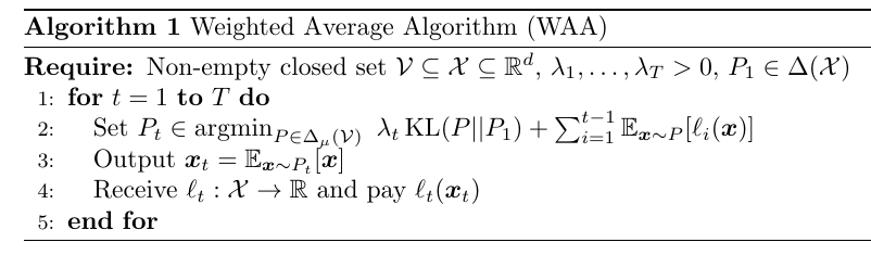
WAA is stated in Algorithm 1. Essentially, WAA predicts with a weighted average of predictions—hence the name of the algorithm—where the weights are proportional to the negative exponential of the cumulative losses of each predictor.

Remark 1. Note that if ${{\boldsymbol u}}$ is such that ${ P_1(\mathrm{d}{\boldsymbol u})=0}$ , then ${P_t(d{\boldsymbol u})=0}$ for all ${t}$ . Hence, if ${P_1 \in \Delta(\mathcal{V})}$ , then ${P_t \in \Delta(\mathcal{V})}$ for all ${t}$ and the constraint to have ${P \in \Delta_\mu(\mathcal{V})}$ is automatically satisfied.

Remark 2. If the losses are convex, predicting with the average instead of sampling makes sense because by Jensen’s inequality, we have

$\displaystyle \ell_t({\boldsymbol x}_t) \leq \mathop{\mathbb E}_{{\boldsymbol x} \sim P_t} [\ell_t({\boldsymbol x})]~.$

Next, we will dig deeper in the concept of exp-concavity that will be used as a key assumption on the losses.

2.1. Convex Analysis Bits: Exp-concavity

Definition 1. Let ${\mathcal{V} \subseteq R^d}$ and ${\alpha>0}$ . A function ${f:\mathcal{V}\rightarrow{\mathbb R}}$ is called ${\alpha}$ ‑exp‑concave if

$\displaystyle x\mapsto e^{-\alpha f(x)}$

is a concave function on ${\mathcal{V}}$ .

Proposition 2. Let ${\alpha >0}$ . If ${f:\mathcal{V} \rightarrow {\mathbb R}}$ is ${\alpha}$ -exp-concave, then ${f}$ is ${\beta}$ -exp-concave for any ${0<\beta<\alpha}$ .

Proof: Observe that ${h({\boldsymbol x})=\exp(-\beta f({\boldsymbol x}))= (\exp(-\alpha f({\boldsymbol x})))^{\beta/\alpha}}$ and ${\exp(-\alpha f({\boldsymbol x}))}$ is non-negative. Hence, we have a composition of a concave function with an increasing concave function. Hence, ${h}$ is concave. $\Box$

Proposition 3. Assume ${f:\mathcal{V}\subseteq R^d \rightarrow{\mathbb R}}$ is ${\alpha}$ -exp-concave and let ${h({\boldsymbol x}) = f({\boldsymbol A} {\boldsymbol x} +{\boldsymbol u})}$ where ${{\boldsymbol A} \in {\mathbb R}^{n \times d}}$ and ${{\boldsymbol u} \in {\mathbb R}^n}$ . Then, ${h}$ is ${\alpha}$ -exp-concave.

Proof: Since ${\exp(-\alpha f({\boldsymbol x}))}$ is concave, then ${\exp(-\alpha h({\boldsymbol x})) = \exp(-\alpha f({\boldsymbol A} {\boldsymbol x}+{\boldsymbol u}))}$ is also concave because it is the composition of a concave function with an affine transformation. $\Box$

The next proposition shows that exp-concavity is a stronger property than convexity.

Proposition 4. Let ${f:\mathcal{V}\rightarrow{\mathbb R}}$ be ${\alpha}$ ‑exp‑concave. Then, ${f}$ is convex.

Proof: Let ${g({\boldsymbol x})=e^{-\alpha f({\boldsymbol x})}}$ . By hypothesis ${g}$ is concave on ${\mathcal V}$ and ${g({\boldsymbol x})>0}$ for all ${{\boldsymbol x}}$ (since the exponential is positive). Fix ${{\boldsymbol x},{\boldsymbol y}\in\mathcal{V}}$ and ${t\in[0,1]}$ . Concavity of ${g}$ gives

$\displaystyle g(t {\boldsymbol x}+(1-t) {\boldsymbol y}) \ge t\,g({\boldsymbol x})+(1-t)\,g({\boldsymbol y})~.$

For the positive numbers ${g({\boldsymbol x}),g({\boldsymbol y})}$ the weighted AM–GM inequality yields

$\displaystyle t\,g({\boldsymbol x})+(1-t)\,g({\boldsymbol y}) \ge g({\boldsymbol x})^t g({\boldsymbol y})^{1-t}~.$

Combining the two inequalities,

$\displaystyle e^{-\alpha f(t {\boldsymbol x}+(1-t) {\boldsymbol y})} =g(t {\boldsymbol x}+(1-t){\boldsymbol y}) \ge g({\boldsymbol x})^t g({\boldsymbol y})^{1-t} = e^{-\alpha\left(t f({\boldsymbol x})+(1-t)f({\boldsymbol y})\right)}~.$

Taking ${-\frac{1}{\alpha}\ln}$ of both sides, yields

$\displaystyle f(t {\boldsymbol x}+(1-t) {\boldsymbol y}) \le t f({\boldsymbol x})+(1-t)f({\boldsymbol y}),$

so ${f}$ is convex. $\Box$

We can also characterize the exp-concavity in terms of the Hessian of a twice differentiable function.

Theorem 5. Let ${f:{\mathbb R}^d \rightarrow {\mathbb R}}$ twice-differentiable. Then, f is ${\alpha}$ -exp-concave iff

$\displaystyle \nabla^2 f(x) \succeq \alpha \nabla f(x)\,\nabla f(x)^\top, \quad\text{for all }x\in{\mathbb R}^d~.$

Proof: The concavity of ${g(x)=e^{-\alpha f(x)}}$ is equivalent to its Hessian being negative semi‑definite: ${\nabla^2 g(x)\preceq 0}$ .

Let’s compute ${\nabla g}$ and ${\nabla^2 g}$ . Denote ${g(x)=e^{-\alpha f(x)}}$ . The gradient is

$\displaystyle \nabla g(x) =\nabla\bigl(e^{-\alpha f(x)}\bigr) =-\alpha\,e^{-\alpha f(x)}\,\nabla f(x)~.$

The Hessian is

$\displaystyle \begin{aligned} \nabla^2 g(x) &=\nabla\bigl(-\alpha e^{-\alpha f(x)}\,\nabla f(x)\bigr)\\ &=-\alpha\,\nabla\bigl(e^{-\alpha f(x)}\bigr)\,\nabla f(x)^\top \;-\;\alpha\,e^{-\alpha f(x)}\,\nabla^2 f(x)\\ &=\;\alpha^2e^{-\alpha f(x)}\,\bigl(\nabla f(x)\nabla f(x)^\top\bigr) \;-\;\alpha e^{-\alpha f(x)}\,\nabla^2 f(x)~. \end{aligned}$

Re‑ordering,

$\displaystyle \nabla^2 g(x) =e^{-\alpha f(x)}\left(\alpha^2\,\nabla f(x)\nabla f(x)^\top \;-\;\alpha\,\nabla^2 f(x)\right)~.$

Since ${e^{-\alpha f(x)}>0}$ and ${\alpha>0}$ , the condition ${\nabla^2g(x)\preceq0}$ is equivalent to ${\alpha\,\nabla f(x)\nabla f(x)^\top \preceq \nabla^2 f(x)}$ . $\Box$

Example 1. Consider ${\mathcal{V}=\{{\boldsymbol x}: \|{\boldsymbol x}\|_2\leq R\}}$ , ${\mathcal{Y}=\{{\boldsymbol y}: \|{\boldsymbol y}\|\leq R\}}$ , and ${f:\mathcal{V} \rightarrow {\mathbb R}}$ defined as ${f({\boldsymbol x})=\|{\boldsymbol x}-{\boldsymbol y}\|_2^2}$ , where ${{\boldsymbol y} \in \mathcal{Y}}$ . We have

$\displaystyle \nabla^2 f({\boldsymbol x})=2 {\boldsymbol I}_d$

and

$\displaystyle \nabla f({\boldsymbol x})=2 ({\boldsymbol x}-{\boldsymbol y})~.$

Using Theorem 5, ${f}$ is ${\alpha}$ -exp-concave iff

$\displaystyle {\boldsymbol I}_d \succeq 2 \alpha ({\boldsymbol x}-{\boldsymbol y})({\boldsymbol x}-{\boldsymbol y})^\top, \ \forall {\boldsymbol x} \in \mathcal{V}, {\boldsymbol y} \in \mathcal{Y}~.$

Hence, we have that ${\alpha=\frac{1}{2(2R)^2}}$ .

Finally, we show that exp-concavity holds on the entire ${{\mathbb R}^d}$ only for constant functions.

Proposition 6. Let ${f:{\mathbb R}^d \rightarrow {\mathbb R}}$ be ${\alpha}$ -exp-concave on ${{\mathbb R}^d}$ . Then, ${f}$ is a constant function.

Proof: Denote by ${h({\boldsymbol x})=-\exp(-\alpha f({\boldsymbol x}))}$ that is convex by definition and it is upper bounded by 0. Suppose that ${h}$ is not constant, this means that there exist ${{\boldsymbol x}, {\boldsymbol y} \in {\mathbb R}^d}$ such that ${h({\boldsymbol x})>h({\boldsymbol y})}$ . Since ${h}$ is convex, we have

$\displaystyle h({\boldsymbol x}) \leq \lambda h\left(\frac{{\boldsymbol x}-(1-\lambda){\boldsymbol y}}{\lambda}\right) + (1-\lambda)h({\boldsymbol y}), \quad \forall \lambda \in (0,1)~.$

Hence, we have

$\displaystyle \frac{h({\boldsymbol x})-h({\boldsymbol y})}{\lambda}+ h({\boldsymbol y}) =\frac{h({\boldsymbol x})-(1-\lambda)h({\boldsymbol y})}{\lambda} \leq h\left(\frac{{\boldsymbol x}-(1-\lambda){\boldsymbol y}}{\lambda}\right) \leq 0~.$

Since ${h({\boldsymbol x})> h({\boldsymbol y})}$ we have that the left hand side of the inequality goes to infinity as ${\lambda \rightarrow 0^+}$ giving a contradiction. Hence, ${h}$ is constant that implies that ${f}$ is constant. $\Box$

Remark 3. The previous result and the fact that exp-concave functions are often used only on bounded domains might induce someone to think that exp-concave function only exists on bounded domains. This is not true: There exists exp-concave ${f:\mathcal{V}\rightarrow {\mathbb R}}$ , where ${\mathcal{V}\subseteq {\mathbb R}^d}$ is not bounded. For example, let ${\mathcal{V}=\{x: x\geq 0\}}$ and ${f(x)= -\ln(x+1)}$ that is 1-exp-concave.

2.2. Analysis of WAA

We now state the regret guarantee for WAA.

Theorem 7. Assume that ${\ell_t}$ to be ${\alpha}$ -exp-concave for all ${t}$ , and ${\frac{1}{\alpha}<\lambda_{t}\leq \lambda_{t+1}}$ for all ${t}$ in Algorithm 2. Then, we have

$\displaystyle \sum_{t=1}^T \ell_t( {\boldsymbol x}_t) \leq \mathop{\mathbb E}_{{\boldsymbol x} \sim Q}\left[\sum_{t=1}^T \ell_t({\boldsymbol x})\right] + \lambda_T \text{KL}(Q||P_1), \quad \forall Q \in \Delta_\mu(\mathcal{V})~.$

Moreover, if ${P_1\in \Delta(\mathcal{V})}$ , we also have

$\displaystyle \sum_{t=1}^T \ell_t( {\boldsymbol x}_t) \leq -\lambda_T \ln \mathop{\mathbb E}_{{\boldsymbol x} \sim P_1}\left[ \exp\left(-\frac{1}{\lambda_T} \sum_{t=1}^T \ell_t({\boldsymbol x})\right)\right]~.$

Proof: We start from (1).

First of all, observe that it holds that (proof left as an exercise)

$\displaystyle \label{eq:aa_alternate_term} \inf_{P} \ \langle f, P\rangle + \lambda \text{KL}(P,Q) = - \lambda \ln \mathop{\mathbb E}_{{\boldsymbol x} \sim Q}\left[\exp\left(- \frac{1}{\lambda} f({\boldsymbol x})\right)\right]~. \ \ \ \ \ (2)$

Given that ${\psi_t(P)=\lambda_t\text{KL}(P||P_1)}$ , we have ${B_{\psi_t}(P;Q) = \lambda_t\text{KL}(P||Q)}$ , because the term depending on ${P_1}$ is constant w.r.t. ${P}$ .

Assuming ${\frac{1}{\lambda_t}}$ non-increasing, we have

$\displaystyle \begin{aligned} F_t(P_t) - F_{t+1}(P_{t+1}) &\leq - \langle\ell_t, P_{t+1}\rangle-B_{F_t}(P_{t+1};P_t) = - \langle \ell_t,P_{t+1}\rangle-B_{\psi_t}(P_{t+1};P_t) \\ &\leq \max_{P} \ - \langle\ell_t,P\rangle-B_{\psi_t}(P;P_t) = \lambda_t\ln \mathop{\mathbb E}_{{\boldsymbol x} \sim P_{t}} \left[\exp\left(-\frac{1}{\lambda_t} \ell_t({\boldsymbol x})\right)\right], \end{aligned}$

where in the first equality we used the fact that the terms with the losses are linear with respect to the distribution, and in the last equality we used (2).

Finally, if ${\ell_t}$ is ${\alpha}$ -exp-concave, using Jensen’s inequality we have

$\displaystyle \lambda_t\ln \mathop{\mathbb E}_{{\boldsymbol x} \sim P_t} \left[\exp\left(-\frac{1}{\lambda_t} \ell_t({\boldsymbol x})\right)\right] + \ell_t\left({\boldsymbol x}_t\right) =\lambda_t\ln \mathop{\mathbb E}_{{\boldsymbol x} \sim P_t} \left[\exp\left(-\frac{1}{\lambda_t} \ell_t({\boldsymbol x})\right)\right] + \ell_t\left(\mathop{\mathbb E}_{{\boldsymbol x} \sim P_t}[{\boldsymbol x}]\right) \leq0,$

for all ${\frac{1}{\lambda_t} \leq \alpha}$ . Putting all together and observing that the last term in (1) is negative for all ${Q \in \Delta_{\mu}(\mathcal{V})}$ , we obtained the first stated bound.

The second bound is obtained by choosing ${Q}$ to minimize ${\mathop{\mathbb E}_{{\boldsymbol x} \sim Q}\left[\sum_{t=1}^T \ell_t({\boldsymbol x})\right] + \lambda_T \text{KL}(Q||P_1)}$ . In this case, the assumption of ${P_1}$ supported on ${\mathcal{V}}$ makes sure that the last term in (1) is negative. $\Box$

So, the WAA algorithm has the surprising property to have a \emph{constant} regret on exp-concave losses with respect to a stochastic competitor.
Unfortunately, the update in the WAA has not a closed formula. In fact, it requires the numerical evaluation of the expectation. However, if the distribution is discrete we can always calculate the prediction.

Example 2. As a practical example, consider the case that ${\mathcal{X}=\mathcal{V}}$ is composed by ${k}$ vectors in ${{\mathbb R}^d}$ , ${\{{\boldsymbol u}_1, \dots, {\boldsymbol u}_k\}}$ . In this case, we have that

$\displaystyle \sum_{t=1}^T \ell_t({\boldsymbol x}_t) = \sum_{t=1}^T \ell_t\left(\sum_{i=1}^k {\boldsymbol x}_i P_{t,i}\right) \leq \min_i \ \sum_{t=1}^T \ell_t({\boldsymbol u}_i) + \lambda_T \ln \frac{1}{P_{1,i}} ~.$

We have proved an upper bound to the regret of WAA that uses a randomized comparator, that is, ${\mathop{\mathbb E}_{{\boldsymbol x} \sim Q}\left[\sum_{t=1}^T \ell_t({\boldsymbol x})\right]}$ . However, sometimes one would like to prove an upper bound that depends on a deterministic one. Hence, now we show how to link the performance of the stochastic comparator to the performance of a deterministic one.

Theorem 8. Assume that ${\mathcal{V}\subseteq {\mathbb R}^d}$ is a convex closed bounded set and set ${P_1}$ to be the uniform distribution on it. Assume that the losses ${\ell_t}$ are ${\alpha}$ -exp-concave and set ${\frac{1}{\lambda_t}=\alpha}$ . Then, Algorithm 2 satisfies

$\displaystyle \label{eq:waa_uniform} \sum_{t=1}^T (\ell_t({\boldsymbol x}_t) - \ell_t({\boldsymbol u})) \leq \frac{d}{\alpha} \left[1+\ln(T/d+1)\right], \ \forall {\boldsymbol u} \in \mathcal{V}~. \ \ \ \ \ (3)$

Proof: Fix ${{\boldsymbol u} \in \mathcal{V}}$ , and define ${\mathcal{V}'=\{{\boldsymbol x} \in {\mathbb R}^d: {\boldsymbol x}=\frac{T/d}{T/d+1}{\boldsymbol u} + \frac{1}{T/d+1}{\boldsymbol w}, {\boldsymbol w} \in \mathcal{V}\} \subseteq \mathcal{V}}$ . Choose ${Q=\frac{1}{\beta} P_1}$ in ${\mathcal{V}'}$ and 0 otherwise, where ${\beta=\int_{\mathcal{V}'} d P_1({\boldsymbol x})}$ .

By the exp-concavity of ${\ell_t}$ , we have for any ${{\boldsymbol x} \in \mathcal{V}'}$

$\displaystyle \exp(-\alpha \ell_t({\boldsymbol x})) \geq \frac{T/d}{T/d+1}\exp(-\alpha \ell_t({\boldsymbol u})) +\frac{1}{T/d+1}\exp(-\alpha \ell_t({\boldsymbol w})) \geq \frac{T/d}{T/d+1}\exp(-\alpha \ell_t({\boldsymbol u}))~.$

Hence, we have for any ${{\boldsymbol x} \in \mathcal{V}'}$

$\displaystyle \exp\left(-\alpha \sum_{t=1}^T \ell_t({\boldsymbol x})\right) \geq \left(\frac{T/d}{T/d+1}\right)^T \exp\left(-\alpha \sum_{t=1}^T \ell_t({\boldsymbol u})\right) \geq \frac{1}{e^d} \exp\left(-\alpha \sum_{t=1}^T \ell_t({\boldsymbol u})\right),$

that implies

$\displaystyle \sum_{t=1}^T \mathop{\mathbb E}_{{\boldsymbol x} \sim Q} [\ell_t({\boldsymbol x})] \leq \frac{d}{\alpha}+ \sum_{t=1}^T \ell_t({\boldsymbol u})~.$

Moreover, the KL term becomes

$\displaystyle \text{KL}(Q||P_1) = \int_{\mathcal{V}} \ln\frac{Q(\mathrm{d} {\boldsymbol x})}{P_1(\mathrm{d} {\boldsymbol x})} Q(\mathrm{d} {\boldsymbol x}) = -\ln \beta = -\ln \int_{\mathcal{V}'} P_1(\mathrm{d} {\boldsymbol x})~.$

Given that ${P_1}$ is uniform on ${\mathcal{V}}$ , we have that

$\displaystyle \int_{\mathcal{V}'} dP_1({\boldsymbol x}) = \frac{Vol(\mathcal{V}')}{Vol(\mathcal{V})} = \frac{1}{(T/d+1)^d},$

because ${\mathcal{V}'}$ is a scaling and translation of ${\mathcal{V}}$ .

Using Theorem 7 and putting all together, we have the stated bound. $\Box$

2.3. ONS and OSD as instantiations of WAA

In this section, we show that WAA is more general than one might think. In fact, we will show that it can be equivalent to online subgradient descent and to the Online Newton Step.

Here, we will set ${\mathcal{X}={\mathbb R}^d}$ and ${P_1}$ as the Gaussian distribution ${\mathcal{N}({\boldsymbol x}_1, {\boldsymbol \Sigma}_1)}$ , where ${{\boldsymbol x}_1 \in \mathcal{V}}$ and ${{\boldsymbol \Sigma}_1\succ 0}$ .

The losses we use are ${\hat{\ell}_t({\boldsymbol x}):=\langle{\boldsymbol g}_t, {\boldsymbol x}\rangle+\frac12 \|{\boldsymbol x}-{\boldsymbol x}_t\|^2_{{\boldsymbol M}_t}}$ . Hence, we have

$\displaystyle P_t = \mathop{\mathrm{argmin}}_{P \in \Delta_\mu(\mathcal{V})} \ \text{KL}(P||\hat{P}_t) = \mathcal{N}({\boldsymbol x}_t, {\boldsymbol \Sigma}_t)~.$

where

$\displaystyle \begin{aligned} {\boldsymbol x}_t &= \mathop{\mathrm{argmin}}_{{\boldsymbol x} \in \mathcal{V}} \ ({\boldsymbol x}-\hat{{\boldsymbol x}}_t)^\top {\boldsymbol \Sigma}^{-1}_{t}({\boldsymbol x}-\hat{{\boldsymbol x}}_t),\\ \hat{P}_t(\mathrm{d} {\boldsymbol x})& \propto\exp\left(-\frac12\|{\boldsymbol x}-{\boldsymbol x}_1\|_{{\boldsymbol \Sigma}_1}^2-\frac{1}{\lambda} \sum_{i=1}^{t-1}\left(\langle {\boldsymbol g}_i, {\boldsymbol x}\rangle +\frac12 \|{\boldsymbol x}-{\boldsymbol x}_i\|_{{\boldsymbol M}_i}^2\right)\right) = \mathcal{N}\left(\hat{{\boldsymbol x}}_t, {\boldsymbol \Sigma}_t\right), \end{aligned}$

and ${\hat{{\boldsymbol x}}_t={\boldsymbol \Sigma}_{t}\left({\boldsymbol \Sigma}_1^{-1} {\boldsymbol x}_1+\frac{1}{\lambda}\sum_{i=1}^{t-1} ({\boldsymbol M}_i {\boldsymbol x}_i-{\boldsymbol g}_i)\right)}$ and ${{\boldsymbol \Sigma}_{t}=\left({\boldsymbol \Sigma}_1^{-1}+\frac{1}{\lambda} \sum_{i=1}^{t-1} {\boldsymbol M}_i\right)^{-1}}$ . From the above, we clearly have ${{\boldsymbol x}_t=\mathop{\mathbb E}_{{\boldsymbol x} \sim P_t}[{\boldsymbol x}]}$ .

However, ${{\boldsymbol x}_t}$ can also be written as

$\displaystyle {\boldsymbol x}_t = \mathop{\mathrm{argmin}}_{{\boldsymbol x} \in \mathcal{V}} \ \frac12\|{\boldsymbol x}-{\boldsymbol x}_1\|^2_{{\boldsymbol \Sigma}_1^{-1}}+\frac{1}{\lambda}\sum_{i=1}^{t-1} \left(\langle {\boldsymbol g}_i, {\boldsymbol x}\rangle+ \frac12 \|{\boldsymbol x}-{\boldsymbol x}_i\|_{{\boldsymbol M}_i}^2\right),$

that is, the solution of FTRL with regularizer ${\psi({\boldsymbol x})=\frac12\|{\boldsymbol x}-{\boldsymbol x}_1\|^2_{{\boldsymbol \Sigma}_1^{-1}}}$ on the surrogate losses ${\hat{\ell}_t}$ . This implies that ${{\boldsymbol x}_t}$ is equivalent to the output of the algorithm for weaker notion of strong convexity. So, using the notation ${{\boldsymbol S}_{t}={\boldsymbol \Sigma}_1^{-1}+\frac{1}{\lambda} \sum_{i=1}^{t} {\boldsymbol M}_i}$ , we can directly use the bound we proved for it:

$\displaystyle \sum_{t=1}^T \tilde{\ell}_t({\boldsymbol x}_t) - \sum_{t=1}^T \tilde{\ell}_t({\boldsymbol u}) \leq \frac{1}{2} \|{\boldsymbol u}-{\boldsymbol x}_1\|_{{\boldsymbol \Sigma}^{-1}}^2 -\min_{{\boldsymbol x} \in \mathcal{V}} \ \frac{1}{2} \|{\boldsymbol x}-{\boldsymbol x}_1\|^2_{{\boldsymbol \Sigma}^{-1}} + \frac12 \sum_{t=1}^T \|{\boldsymbol g}_t\|^2_{{\boldsymbol S}^{-1}_t}~.$

Hence, we have the following cases:

For exp-concave losses, we recover the regret upper bound of the ONS algorithm.
For convex losses, we have ${M_t=\boldsymbol{0}}$ . Hence, we have
$\displaystyle \sum_{t=1}^T \ell_t({\boldsymbol x}_t) - \sum_{t=1}^T \ell_t({\boldsymbol u}) \leq \sum_{t=1}^T \tilde{\ell}_t({\boldsymbol x}_t) - \sum_{t=1}^T \tilde{\ell}_t({\boldsymbol u}) \leq \frac{1}{2} \|{\boldsymbol u}-{\boldsymbol x}_1\|_{{\boldsymbol \Sigma}_1^{-1}}^2 -\min_{{\boldsymbol x} \in \mathcal{V}} \ \frac{1}{2} \|{\boldsymbol x}-{\boldsymbol x}_1\|^2_{{\boldsymbol \Sigma}_1^{-1}} + \frac12 \sum_{t=1}^T \|{\boldsymbol g}_t\|^2_{{\boldsymbol \Sigma}_1}~.$

If in addition ${{\boldsymbol \Sigma}_1=\frac{1}{\lambda} {\boldsymbol I}_d}$ , we have

$\displaystyle \sum_{t=1}^T \ell_t({\boldsymbol x}_t) - \sum_{t=1}^T \ell_t({\boldsymbol u}) \leq \sum_{t=1}^T \tilde{\ell}_t({\boldsymbol x}_t) - \sum_{t=1}^T \tilde{\ell}_t({\boldsymbol u}) \leq \frac{\lambda}{2} \|{\boldsymbol x}_1-{\boldsymbol u}\|_2^2 -\min_{{\boldsymbol x} \in \mathcal{V}} \ \frac{\lambda}{2} \|{\boldsymbol x}-{\boldsymbol x}_1\|^2_2 + \frac{1}{2\lambda} \sum_{t=1}^T \|{\boldsymbol g}_t\|^2_2~.$
For ${\beta}$ -strongly losses with respect to ${\|\cdot\|_2}$ , we have ${{\boldsymbol M}_t=\beta {\boldsymbol I}_d}$ . Hence, we can set ${{\boldsymbol \Sigma}^{-1}_1=\boldsymbol{0}}$ and ${\lambda=1}$ to have
$\displaystyle \sum_{t=1}^T \ell_t({\boldsymbol x}_t) - \sum_{t=1}^T \ell_t({\boldsymbol u}) \leq \sum_{t=1}^T \tilde{\ell}_t({\boldsymbol x}_t) - \sum_{t=1}^T \tilde{\ell}_t({\boldsymbol u}) \leq \frac{1}{2} \sum_{t=1}^T \frac{\|{\boldsymbol g}_t\|^2_2}{\beta t}~.$

In the next theorem, we also show that the bound in Theorem 7 is powerful enough to capture all the cases above.

Theorem 9. Let ${\mathcal{X}={\mathbb R}^d}$ and run WAA on the losses ${\hat{\ell}_t({\boldsymbol x}):=\langle{\boldsymbol g}_t, {\boldsymbol x}\rangle+\frac12 \|{\boldsymbol x}-{\boldsymbol x}_t\|^2_{{\boldsymbol M}_t}}$ , where ${{\boldsymbol g}_t \in {\mathbb R}^d}$ and ${{\boldsymbol M}_t \succeq 0}$ are arbitrary for all ${t}$ . Set ${P_1=\mathcal{N}({\boldsymbol x}_1, {\boldsymbol \Sigma}_1)}$ , where ${{\boldsymbol x}_1 \in \mathcal{V}}$ and ${{\boldsymbol \Sigma}_1 \succ 0}$ . Then, we have

$\displaystyle \sum_{t=1}^T \left(\hat{\ell}_t({\boldsymbol x}_t)-\hat{\ell}_t({\boldsymbol u})\right) \leq \frac{\lambda}{2} \|{\boldsymbol x}_1-{\boldsymbol u}\|^2_{{\boldsymbol \Sigma}^{-1}_1} + \frac{1}{2 \lambda}\sum_{t=1}^T \|{\boldsymbol g}_t\|^2_ {{\boldsymbol \Sigma}_{t+1}},$

where ${{\boldsymbol \Sigma}_{t+1}=\left({\boldsymbol \Sigma}_1^{-1}+\frac{1}{\lambda} \sum_{i=1}^{t} {\boldsymbol M}_i\right)^{-1}}$ for all ${t}$ .

Proof: Select ${Q=\mathcal{N}({\boldsymbol u}, {\boldsymbol C})}$ for any ${{\boldsymbol u} \in \mathcal{V}}$ and we will specify ${{\boldsymbol C}}$ in the following.

Observe that the quadratic nature of the losses allows us to easily go from a stochastic to a deterministic competitor:

$\displaystyle \mathop{\mathbb E}_{{\boldsymbol x} \sim Q}[\hat{\ell}_t({\boldsymbol x})] = \ell_t({\boldsymbol x}_t)+\langle {\boldsymbol g}_t, {\boldsymbol u}-{\boldsymbol x}_t\rangle + \frac12\text{Tr}[{\boldsymbol C} {\boldsymbol M}_t]+ \frac12 \|{\boldsymbol u}-{\boldsymbol x}_t\|^2_{{\boldsymbol M}_t} = \hat{\ell}_t({\boldsymbol u})+\frac12 \text{Tr}[{\boldsymbol C} {\boldsymbol M}_t]~.$

Hence, we have

$\displaystyle \sum_{t=1}^T \left(\ell_t({\boldsymbol x}_t)-\ell_t({\boldsymbol u})\right) \leq \sum_{t=1}^T \left(\hat{\ell}_t({\boldsymbol x}_t)-\hat{\ell}_t({\boldsymbol u})\right) = \sum_{t=1}^T \left(\hat{\ell}_t({\boldsymbol x}_t)-\mathop{\mathbb E}_{{\boldsymbol x}\sim Q}[\hat{\ell}_t({\boldsymbol x})]\right)+\frac12 \text{Tr}\left({\boldsymbol C} \sum_{t=1}^T {\boldsymbol M}_t\right)~.$

From (1), we have

$\displaystyle \sum_{t=1}^T \left(\hat{\ell}_t({\boldsymbol x}_t)-\mathop{\mathbb E}_{{\boldsymbol x}\sim Q}[\hat{\ell}_t({\boldsymbol x})]\right) \leq \lambda \text{KL}(Q||P_1) + \sum_{t=1}^T \lambda \ln \mathop{\mathbb E}_{{\boldsymbol x}\sim P_t}\left[\exp\left(-\frac{1}{\lambda}\left( \hat{\ell}_t({\boldsymbol x})-\hat{\ell}_t({\boldsymbol x}_t)\right)\right)\right]~.$

From the update rule, we have

$\displaystyle \begin{aligned} \lambda \ln\mathop{\mathbb E}_{{\boldsymbol x}\sim P_t}\left[\exp\left(-\frac{1}{\lambda} \hat{\ell}_t({\boldsymbol x})\right)\right]+\hat{\ell}_t({\boldsymbol x}_t) &=\lambda \ln\mathop{\mathbb E}_{{\boldsymbol x}\sim P_t}\left[\exp\left(-\frac{1}{\lambda} \left(\hat{\ell}_t({\boldsymbol x})-\hat{\ell}_t({\boldsymbol x}_t)\right)\right)\right]\\ &= \lambda \ln\mathop{\mathbb E}_{{\boldsymbol x}\sim P_t}\left[\exp\left(-\frac{1}{\lambda} \left(\langle {\boldsymbol g}_t, {\boldsymbol x}-{\boldsymbol x}_t\rangle + \frac12 \|{\boldsymbol x}-{\boldsymbol x}_t\|^2_{{\boldsymbol M}_t}\right)\right)\right] \\ &= \frac{1}{2 \lambda}{\boldsymbol g}_t^\top {\boldsymbol \Sigma}_{t+1}{\boldsymbol g}_t - \frac{\lambda}{2}\ln \frac{|{\boldsymbol \Sigma}_{t}|}{|{\boldsymbol \Sigma}_{t+1}|}, \end{aligned}$

where in the last inequality we used the that

$\displaystyle \mathop{\mathbb E}_{{\boldsymbol x}\sim \mathcal{N}({\boldsymbol x}_t,{\boldsymbol \Sigma}_t)} \left[\exp\left(-\frac{1}{\lambda}\langle {\boldsymbol g}_t, {\boldsymbol x}-{\boldsymbol x}_t\rangle\right)\right] =\exp\left(\frac{1}{2 \lambda^2}{\boldsymbol g}_t^\top \left({\boldsymbol \Sigma}_t^{-1}+\frac{1}{\lambda} M_t\right)^{-1} {\boldsymbol g}_t\right) =\exp\left(\frac{1}{2 \lambda^2}{\boldsymbol g}_t^\top {\boldsymbol \Sigma}_{t+1}^{-1} {\boldsymbol g}_t\right),$

and ${\mathop{\mathbb E}_{{\boldsymbol x}\sim \mathcal{N}(\boldsymbol{0},{\boldsymbol \Sigma}_t)}[\exp(-\frac{1}{2 \lambda} {\boldsymbol x}^\top {\boldsymbol M}_t {\boldsymbol x})]=\frac{1}{\sqrt{|{\boldsymbol I}_d+\frac{1}{\lambda}{\boldsymbol \Sigma}_t {\boldsymbol M}_t|}}}$ . Finally, we have

$\displaystyle \text{KL}(Q||P_1) = \frac12 \left(\ln\frac{|{\boldsymbol \Sigma}_1|}{|{\boldsymbol C}|}+\text{Tr}({\boldsymbol C} {\boldsymbol \Sigma}^{-1}_1)-d+ ({\boldsymbol x}_1-{\boldsymbol u})^\top {\boldsymbol \Sigma}^{-1}_1({\boldsymbol x}_1-{\boldsymbol u}) \right)~.$

Putting all together, we obtain

$\displaystyle \frac{\lambda}{2} \left(\ln\frac{|{\boldsymbol \Sigma}_1|}{|{\boldsymbol C}|}+\text{Tr}({\boldsymbol C} {\boldsymbol \Sigma}^{-1}_1)-d+ ({\boldsymbol x}_1-{\boldsymbol u})^\top {\boldsymbol \Sigma}^{-1}_1({\boldsymbol x}_1-{\boldsymbol u}) \right) + \frac{1}{2 \lambda}\sum_{t=1}^T {\boldsymbol g}_t^\top {\boldsymbol \Sigma}_{t+1}{\boldsymbol g}_t - \frac{\lambda}{2}\ln \frac{|{\boldsymbol \Sigma}_{1}|}{|{\boldsymbol \Sigma}_{T+1}|} + \frac{1}{2} \text{Tr}\left[C \sum_{t=1}^T {\boldsymbol M}_t\right]~.$

We now select ${{\boldsymbol C}={\boldsymbol \Sigma}_{T+1}=({\boldsymbol \Sigma}_1^{-1}+\frac{1}{\lambda} \sum_{t=1}^T {\boldsymbol M}_t)^{-1}}$ which minimizes the bound, to have

$\displaystyle \begin{aligned} &\frac{\lambda}{2} \left(\ln\frac{|{\boldsymbol \Sigma}_1|}{|{\boldsymbol \Sigma}_{T+1}|}+\text{Tr}({\boldsymbol \Sigma}_{T+1} {\boldsymbol \Sigma}^{-1}_1)-d+ ({\boldsymbol u}-{\boldsymbol x}_1)^\top {\boldsymbol \Sigma}^{-1}_1({\boldsymbol u}-{\boldsymbol x}_1) \right) + \frac{1}{2\lambda}\sum_{t=1}^T {\boldsymbol g}_t^\top {\boldsymbol \Sigma}_{t+1}{\boldsymbol g}_t - \frac{\lambda}{2}\ln \frac{|{\boldsymbol \Sigma}_{1}|}{|{\boldsymbol \Sigma}_{T+1}|}\\ &\quad + \frac{1}{2} \text{Tr}\left[{\boldsymbol \Sigma}_{T+1} \sum_{t=1}^T {\boldsymbol M}_t\right]\\ &=\frac{\lambda}{2} ({\boldsymbol x}_1-{\boldsymbol u})^\top {\boldsymbol \Sigma}^{-1}_1({\boldsymbol x}_1-{\boldsymbol u}) + \frac{1}{2 \lambda}\sum_{t=1}^T {\boldsymbol g}_t^\top {\boldsymbol \Sigma}_{t+1}{\boldsymbol g}_t~. \end{aligned}$

$\Box$

3. Example of WAA: The Krichevsky-Trofimov Betting Algorithm

Here, we show how to derive the Krichevsky-Trofimov betting algorithm and its regret upper bound. We consider the WAA algorithm where we set the losses to ${\ell_t(x)=-\ln(1+c_t x)}$ where ${c_t \in \{-1, 1\}}$ with the feasible set ${\mathcal{V}=[-1,1]}$ . It is immediate to verify that these losses are 1-exp-concave. Finally, we set ${P_1(\mathrm{d} x)=\frac{1}{\pi \sqrt{(1-x)(1+x)}}}$ over ${\mathcal{V}}$ .

Given that ${c_t \in \{-1, 1\}}$ , we define ${a_t=\sum_{i=1}^t \boldsymbol{1}[c_i=1]}$ and ${b_t=\sum_{i=1}^t \boldsymbol{1}[c_i=-1]}$ , to have

$\displaystyle \begin{aligned} \mathop{\mathbb E}_{x \sim P_1}\left[\prod_{i=1}^t (1+c_i x)\right] &= \frac{2^{a_t+b_t} \Gamma(a_t+1/2) \Gamma(b_t+1/2)}{\pi \Gamma(a_t+b_t+1)},\\ \mathop{\mathbb E}_{x \sim P_1}\left[x \prod_{i=1}^t (1+c_i x)\right] &= \frac{2^{a_t+b_t}\, (a_t-b_t) \, \Gamma(a_t+1/2)\, \Gamma(b_t+1/2)}{\pi\, (a_t+b_t+1)\,\Gamma(a_t+b_t+1)},\\ \max_v \ \prod_{t=1}^T (1+c_t v) =\max_v \ (1+v)^{a_T} (1-v)^{b_T} &= \left(1+\frac{a_T-b_T}{T}\right)^{a_T} \left(1-\frac{a_T-b_T}{T}\right)^{b_T} = 2^T a_T^{a_T} b_T^{b_T} T^{-T}~. \end{aligned}$

With the above formulas we can calculate that

$\displaystyle P_{t+1}(\mathrm{d}x)=\frac{\pi\, \Gamma(a_t+b_t+1) \prod_{i=1}^t (1+c_i x) P_1(\mathrm{d} x)}{2^{a_t+b_t}\, \Gamma(a_t+1/2)\, \Gamma(b_t+1/2)},$

and

$\displaystyle x_{t+1} =\mathop{\mathbb E}_{x \sim P_t}[x] =\frac{a_t-b_t}{a_t+b_t+1} =\frac{\sum_{i=1}^t c_i}{t+1}~.$

Using the second result in Theorem 7, we have

$\displaystyle \begin{aligned} \sum_{t=1}^T (\ell_t(x_t)-\ell_t(u)) &\leq \ln \frac{\max_{v \in [-1,1]} \ \prod_{t=1}^T (1+c_t v)}{\mathop{\mathbb E}_{x \sim P_1} [\prod_{t=1}^T (1+c_t x)]}\\ &\leq \ln \frac{2^T a_T^{a_T} b_T^{b_T} T^{-T} \, \pi \, \Gamma(a_T+b_T+1)}{2^{a_T+b_T}\,\Gamma(a_T+1/2) \, \Gamma(b_T+1/2) }\\ &= \ln \frac{a_T^{a_T} b_T^{b_T} T^{-T} \pi \, \Gamma(T+1)}{\Gamma(a_T+1/2) \, \Gamma(b_T+1/2) }~. \end{aligned}$

Using Lemma 13.6 in my draft book, we have that this expression is maximized for ${a_T=T}$ and ${b_T=0}$ (or equivalently ${a_T=0}$ and ${b_T=T}$ ), so we obtain

$\displaystyle \sum_{t=1}^T (\ell_t(x_t)-\ell_t(u)) \leq \ln \frac{\pi \, \Gamma(T+1)}{\Gamma(T+1/2) \, \Gamma(1/2) } = \ln \frac{\sqrt{\pi} \, \Gamma(T+1)}{\Gamma(T+1/2) }~.$

4. History Bits

The WAA is from Kivinen&Warmuth (1999), as a simplification of the AA of Vovk (1990) (see also Vovk (1998, Appendix A) for an easier description of the AA).
This algorithm is known with many names: Cesa-Bianchi&Lugosi (2006) calls it “exponentially weighted mixture forecaster”, Hazan et al. (2006), Hazan et al. (2007) rediscover it (see below) and name it “exponentially weighted online optimization algorithm”, Wouter Koolen calls it simply “exponential weights algorithm” in his blog post in 2016 (see below). I preferred to use the name that its designers gave to it, also because its acronym nicely matches the one of the Aggregating Algorithm.
Theorem 5 and Example 1 are from Kivinen&Warmuth (1999).

The observation that the AA also works for infinite sets of experts was made by Freund (1996), Freund (2003).

Theorem 8 is from Hazan et al. (2006), Hazan et al. (2007), where they seem to rediscover the WAA algorithm with uniform prior, but I improved it by adding ${1/d}$ term in the logarithm. The proof of Hazan et al. (2006), Hazan et al. (2007) is a generalization of the one of Blum&Kalai (1997), Blum&Kalai (1999) for universal portfolio.

Almost the entire Section 2.3 is from a blog post by Wouter Koolen (the blog of Wouter is really good, full of gems and this is one of them!), where it is done for OGD, while I derived it for FTRL. van der Hoeven&van Erven (2016) has extended this equivalence to Online Mirror Descent. The subtlety of defining the prior on ${\mathcal{X}}$ instead than on ${\mathcal{V}}$ is by me and it allows to state a single theorem that covers all the cases.

Acknowledgments
Thanks to Wei-Cheng Lee for feedback on a prelimary version of this post and to Gemini 2.5 for checking all the proofs.

Parameter-free Learning and Optimization Algorithms

The Weighted Average Algorithm

Leave a comment Cancel reply

Share this:

Related

Leave a comment Cancel reply