Follow-The-Regularized-Leader III: More Logarithmic Bounds

This post is part of the lecture notes of my class “Introduction to Online Learning” at Boston University, Fall 2019.

You can find all the lectures I published here.

In this lecture, we will explore the possibility to obtain logarithmic regret for non-strongly convex functions. Also, we explore a bit more the strategy of moving pieces of the losses inside the regularizer, as we did for the composite and strongly convex losses.

1. Online Newton Step

Last time, we saw that the notion of strong convexity allows us to build quadratic surrogate loss functions, on which Follow-The-Regularized-Leader (FTRL) has smaller regret. Can we find a more general notion of strong convexity that allows to get a small regret for a larger class of functions? We can start from strong convexity and try to generalize it. So, instead of asking that the function is strongly convex w.r.t. a norm, we might be happy requiring strong convexity holds in a particular point w.r.t. a norm that depends on the points itself.

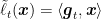
In particular, we can require that for each loss ${\ell_t}$ and for all ${{\boldsymbol x} \in \mathop{\mathrm{dom}} \ell_t}$ the following holds

$\displaystyle \forall {\boldsymbol x} \in V, {\boldsymbol g} \in \partial \ell_t({\boldsymbol x}), \exists A_t \in {\mathbb R}^{d \times d} \ : \ A_t \succeq 0 , \ \ell_t({\boldsymbol y}) \geq \ell_t({\boldsymbol x}) + \langle {\boldsymbol g} , {\boldsymbol y} - {\boldsymbol x} \rangle + \frac{1}{2} \| {\boldsymbol x} - {\boldsymbol y} \|_{A_t}^2, \forall {\boldsymbol y} \in V~.$

where ${\|{\boldsymbol x}\|_{A_t}}$ is defined as ${\sqrt{{\boldsymbol x}^\top A_t{\boldsymbol x}}}$ . Note that this is a weaker property than strong convexity because ${A_t}$ depends on ${{\boldsymbol x}}$ . On the other hand, in the definition of strong convexity we want the last term to be the same norm (or Bregman divergence in the more general formulation) everywhere in the space.

The rationale of this new definition is that it still allows us to build surrogate loss functions, but without requiring to have strong convexity over the entire space. Hence, we can think to use FTRL on the surrogate losses

$\displaystyle \tilde{\ell}_t({\boldsymbol x})=\langle {\boldsymbol g}_t, {\boldsymbol x}\rangle$

and the proximal regularizers ${\psi_t({\boldsymbol x}) = \frac{\lambda}{2} \|{\boldsymbol x}\|^2 + \frac12 \sum_{i=1}^{t-1} \|{\boldsymbol x}_i -{\boldsymbol x}\|_{A_i}^2}$ , where ${\lambda>0}$ . We will denote by ${S_t=\lambda I_d + \sum_{i=1}^t A_i}$ .

Remark 1 Note that ${\|{\boldsymbol x}\|_{S_t}:=\sqrt{{\boldsymbol x}\top S_t {\boldsymbol x}}}$ is a norm because ${S_t}$ is Positive Definite (PD) and ${f({\boldsymbol x}) = \frac{1}{2} {\boldsymbol x}^\top S_t {\boldsymbol x}}$ is ${1}$ -strongly convex w.r.t. ${\|\cdot\|_{S_t}}$ defined as ${\|{\boldsymbol x}\|_{S_t} = \sqrt{{\boldsymbol x}^\top S_t {\boldsymbol x}}}$ (because the Hessian is ${S_t}$ and ${{\boldsymbol x}^\top \nabla^2 f({\boldsymbol y}) {\boldsymbol x} = \|{\boldsymbol x}\|^2_{A_t}}$ ). Also, the dual norm of ${\|\cdot\|_{S_t}}$ is ${\|\cdot\|_{S^{-1}_t}}$ .

From the above remark, we have that the regularizer ${\psi_t({\boldsymbol x})}$ is 1-strongly convex w.r.t ${\|\cdot\|_{S_{t-1}}}$ . Hence, using the FTRL regret guarantee for proximal regularizers, we immediately get the following guarantee

$\displaystyle \begin{aligned} \sum_{t=1}^T \langle {\boldsymbol g}_t, {\boldsymbol x}_t\rangle - \sum_{t=1}^T \langle{\boldsymbol g}_t,{\boldsymbol u}\rangle &=\sum_{t=1}^T \tilde{\ell}_t ({\boldsymbol x}_t) - \sum_{t=1}^T \tilde{\ell}_t({\boldsymbol u}) \\ &\leq \psi_{T+1}({\boldsymbol u}) + \frac12 \sum_{t=1}^T \|{\boldsymbol g}_t\|^2_{S_t^{-1}} + \sum_{t=1}^{T} \left(\psi_t({\boldsymbol x}_t) - \psi_{t+1}({\boldsymbol x}_{t})\right) \\ &= \frac{\lambda}{2} \|{\boldsymbol u}\|^2 + \frac{1}{2} \sum_{t=1}^T\|{\boldsymbol x}_t-{\boldsymbol u}\|^2_{A_t} + \frac12 \sum_{t=1}^T \|{\boldsymbol g}_t\|^2_{S_t^{-1}}~. \end{aligned}$

So, reordering the terms we have

$\displaystyle \label{eq:ons_regret} \sum_{t=1}^T \ell_t({\boldsymbol x}_t) - \sum_{t=1}^T \ell_t({\boldsymbol u}) \leq \sum_{t=1}^T \left(\langle {\boldsymbol g}_t, {\boldsymbol x}_t-{\boldsymbol u}\rangle - \frac{1}{2}\|{\boldsymbol u}-{\boldsymbol x}_t\|^2_{A_t}\right) \leq \frac{\lambda}{2} \|{\boldsymbol u}\|^2 + \frac12 \sum_{t=1}^T \|{\boldsymbol g}_t\|^2_{S^{-1}_t}~. \ \ \ \ \ (1)$

Note how the proof and the algorithm mirror what we did in FTRL with strongly convex losses in the last lecture.

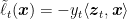
Remark 2 It is possible to generalize our Lemma of FTRL for proximal regularizers to hold in this generalized notion of strong convexity. This would allow to get exactly the same bound running FTRL over the original losses with regularizer ${\psi({\boldsymbol x})=\frac{\lambda}{2}\|{\boldsymbol x}\|_2^2}$ .

Let’s now see a practical instantiation of this idea. Consider the case that the sequence of loss functions we receive satisfy

$\displaystyle \label{eq:exp_concave} \ell_t({\boldsymbol x}) - \ell_t({\boldsymbol u}) \leq \langle {\boldsymbol g}, {\boldsymbol x}-{\boldsymbol u}\rangle -\frac{\mu}{2}(\langle {\boldsymbol g}, {\boldsymbol x}-{\boldsymbol u}\rangle)^2, \ \forall {\boldsymbol x}, {\boldsymbol u} \in V, {\boldsymbol g} \in \partial \ell_t({\boldsymbol x})~. \ \ \ \ \ (2)$

In words, we assume to have a class of functions that can be lower bounded by a quadratic that depends on the current subgradient. In particular, these functions posses some curvature only in the direction of (any of) the subgradients. Denoting by ${A_t= \mu {\boldsymbol g}_t {\boldsymbol g}_t^\top}$ , we can use the above idea using

$\displaystyle \psi_{t}({\boldsymbol x}) =\frac{\lambda}{2} \|{\boldsymbol x}\|^2 + \frac12 \sum_{i=1}^{t-1} \|{\boldsymbol x}_i -{\boldsymbol x}\|_{A_i}^2 = \frac{\lambda}{2} \|{\boldsymbol x}\|^2 + \frac{\mu}{2} \sum_{i=1}^{t-1} (\langle{\boldsymbol g}_i,{\boldsymbol x}-{\boldsymbol x}_i\rangle)^2~.$

Hence, the update rule would be

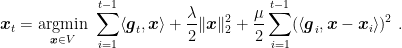
$\displaystyle {\boldsymbol x}_{t} = \mathop{\mathrm{argmin}}_{{\boldsymbol x} \in V} \ \sum_{i=1}^{t-1} \langle {\boldsymbol g}_t, {\boldsymbol x}\rangle + \frac{\lambda }{2}\|{\boldsymbol x}\|_2^2 + \frac{\mu}{2} \sum_{i=1}^{t-1} (\langle{\boldsymbol g}_i,{\boldsymbol x}-{\boldsymbol x}_i\rangle)^2~.$

We obtain the following algorithm, called Online Newton Step (ONS).

ons

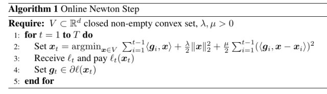
Denoting by 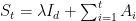${S_t=\lambda I_d + \sum_{i=1}^{t} A_i}$ and using (1), we have

$\displaystyle \sum_{t=1}^T \ell_t({\boldsymbol x}_t) - \sum_{t=1}^T \ell_t({\boldsymbol u}) \leq \frac{\lambda }{2} \|{\boldsymbol u}\|_2^2 + \frac12 \sum_{t=1}^T \|{\boldsymbol g}_t\|^2_{S^{-1}_t}~.$

To bound the last term, we will use the following Lemma.

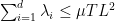
Lemma 1 (Cesa-Bianchi, N. and Lugosi, G. , 2006, Lemma 11.11 and Theorem 11.7) Let ${{\boldsymbol z}_1,\dots, {\boldsymbol z}_T}$ a sequence of vectors in ${{\mathbb R}^d}$ and ${\lambda>0}$ . Define ${H_t=\lambda I_d + \sum_{i=1}^t {\boldsymbol z}_i {\boldsymbol z}_i^\top}$ . Then, the following holds

$\displaystyle \sum_{t=1}^T {\boldsymbol z}_t^\top H_t^{-1} {\boldsymbol z}_t \leq \sum_{i=1}^d \ln \left(1 + \frac{\lambda_i}{\lambda}\right),$

where ${\lambda_1, \dots, \lambda_d}$ are the eigenvalues of ${H_T-\lambda I_d}$ .

Putting all together and assuming ${\|{\boldsymbol g}_t\|_2\leq L}$ and (2) holds for the losses, then ONS satisfies the following regret

$\displaystyle \sum_{t=1}^T \ell_t({\boldsymbol x}_t) - \sum_{t=1}^T \ell_t({\boldsymbol u}) \leq \frac{\lambda }{2} \|{\boldsymbol u}\|_2^2 + \frac{1}{2\mu} \sum_{i=1}^d \ln \left(1+\frac{\lambda_i}{\lambda}\right) \leq \frac{\lambda }{2} \|{\boldsymbol u}\|_2^2 + \frac{d}{2\mu}\ln \left(1 + \frac{\mu T L^2}{d \lambda }\right),$

where in the second inequality we used the inequality of arithmetic and geometric means, 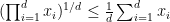${(\prod_{i=1}^d x_i)^{1/d} \leq \frac{1}{d} \sum_{i=1}^d x_i}$ , and the fact that ${\sum_{i=1}^d \lambda_i \leq \mu TL^2}$ .

Hence, if the losses satisfy (2), we can guarantee a logarithmic regret. However, differently from the strongly convex case, here the complexity of the update is at least quadratic in the number of dimensions. Moreover, the regret also depends linearly on the number of dimensions.

Remark 3 Despite the name, the ONS algorithm should not be confused with the Netwon algorithm. They are similar in spirit because they both construct quadratic approximation to the function, but the Netwon algorithm uses the exact Hessian while the ONS uses an approximation that works only for a restricted class of functions. In this view, the ONS algorithm is more similar to Quasi-Newton methods.

Let’s now see an example of functions that satisfy (2).

Example 1 (Exp-Concave Losses) Defining ${X\subseteq{\mathbb R}^d}$ convex, we say that a function ${f:X\rightarrow {\mathbb R}}$ is ${\alpha}$ -exp-concave if ${\exp(-\alpha f({\boldsymbol x}))}$ is concave.

Choose ${\beta \leq \frac{\alpha}{2}}$ such that ${|\beta \langle {\boldsymbol g}, {\boldsymbol y} -{\boldsymbol x}\rangle| \leq \frac{1}{2}}$ for all ${{\boldsymbol x}, {\boldsymbol y} \in X}$ and ${{\boldsymbol g} \in \partial f({\boldsymbol x})}$ . Note that we need a bounded domain for ${\beta}$ to exist. Then, this class of functions satisfy the property (2). In fact, given that ${f}$ is ${\alpha}$ -exp-concave then it is also ${2 \beta}$ -exp-concave. Hence, from the definition we have

$\displaystyle \exp(-2 \beta f({\boldsymbol y})) \leq \exp(-2 \beta f({\boldsymbol x})) - 2\beta \exp(-2 \beta f({\boldsymbol x})) \langle {\boldsymbol g}, {\boldsymbol y} -{\boldsymbol x}\rangle,$

that is

$\displaystyle \exp(-2 \beta f({\boldsymbol y})+ 2\beta f({\boldsymbol x})) \leq 1 - 2 \beta \langle {\boldsymbol g}, {\boldsymbol y} -{\boldsymbol x}\rangle,$

that implies

$\displaystyle f({\boldsymbol x}) - f({\boldsymbol y}) \leq \frac{1}{2\beta}\ln \left( 1+ 2 \beta \langle {\boldsymbol g}, {\boldsymbol x}- {\boldsymbol y}\rangle\right) \\ \leq \langle {\boldsymbol g}, {\boldsymbol x}- {\boldsymbol y}\rangle - \frac{\beta}{2} (\langle {\boldsymbol g}, {\boldsymbol y} -{\boldsymbol x}\rangle)^2,$

where we used the elementary inequality ${\ln(1+x)\leq x - x^2/4}$ , for ${|x|\leq 1}$ .

Example 2 Let ${V=\{{\boldsymbol x} \in {\mathbb R}^d: \|{\boldsymbol x}\|\leq U\}}$ . The logistic loss of a linear predictor ${\ell({\boldsymbol x})= \ln (1+\exp(-\langle {\boldsymbol z},{\boldsymbol x}\rangle))}$ , where ${\|{\boldsymbol z}\|_2\leq 1}$ is ${\exp(-2U)/2}$ -exp-concave.

2. Online Regression: Vovk-Azoury-Warmuth Forecaster

Let’s now consider the specific case that ${\ell_t({\boldsymbol x})=\frac12 (\langle {\boldsymbol z}_t, {\boldsymbol x}\rangle - y_t)^2}$ and ${V={\mathbb R}^d}$ , that is the one of unconstrained online linear regression with square loss. These losses are not strongly convex w.r.t. ${{\boldsymbol x}}$ , but they are exp-concave when the domain is bounded. We could use the ONS algorithm, but it would not work in the unbounded case. Another possibility would be to run FTRL, but that losses are not strongly convex and we would get only a ${O(\sqrt{T})}$ regret.

It turns out we can still get a logarithmic regret, if we make an additional assumption! We will assume to have access to ${{\boldsymbol z}_t}$ before predicting ${{\boldsymbol x}_t}$ . Note that this is a mild assumptions in most of the interesting applications. Then, the algorithm will just be FTRL over the past losses plus the loss on the received ${{\boldsymbol z}_t}$ hallucinating a label of ${0}$ . This algorithm is called Vovk-Azoury-Warmuth from the name of the inventors. The details are in Algorithm 2.

vaw

As we did for composite losses, we look closely to the loss functions, to see if there are terms that we might move inside the regularizer. The motivation would be the same as in the composite losses case: the bound will depends only on the subgradients of the part of the losses that are outside of the regularizer.

So, observe that

$\displaystyle \ell_t({\boldsymbol x})= \frac12 (\langle {\boldsymbol z}_t, {\boldsymbol x}\rangle)^2 - y_t \langle {\boldsymbol z}_t, {\boldsymbol x}\rangle + \frac12 y_t^2~.$

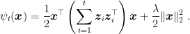
From the above, we see that we could think to move the terms ${\frac12(\langle {\boldsymbol z}_t, {\boldsymbol x}_t\rangle)^2}$ in the regularizer and leaving the linear terms in the loss: ${\tilde{\ell}_t({\boldsymbol x})=- y_t \langle {\boldsymbol z}_t, {\boldsymbol x}\rangle}$ . Hence, we will use

$\displaystyle \psi_t({\boldsymbol x}) = \frac{1}{2}{\boldsymbol x}^\top \left(\sum_{i=1}^t {\boldsymbol z}_i {\boldsymbol z}_i^\top\right){\boldsymbol x} + \frac{\lambda}{2}\|{\boldsymbol x}\|_2^2~.$

Note that the regularizer at time ${t}$ contains the ${{\boldsymbol z}_t}$ that is revealed to the algorithm before it makes its prediction. For simplicity of notation, denote by ${S_t=\lambda I_d +\sum_{i=1}^t {\boldsymbol z}_i {\boldsymbol z}_i^\top}$ .

Using such procedure, the prediction can be written in a closed form:

$\displaystyle \begin{aligned} {\boldsymbol x}_t &= \mathop{\mathrm{argmin}}_{{\boldsymbol x}} \ \frac{\lambda}{2}\|{\boldsymbol x}\|^2_2 + \frac12 \sum_{i=1}^{t-1} (\langle {\boldsymbol z}_i,{\boldsymbol x}\rangle - y_i)^2 + \frac12 (\langle {\boldsymbol z}_t,{\boldsymbol x}\rangle)^2 \\ &= \left(\lambda I_d + \sum_{i=1}^t {\boldsymbol z}_i {\boldsymbol z}_i^\top\right)^{-1} \sum_{i=1}^{t-1} y_i {\boldsymbol z}_i ~. \end{aligned}$

Hence, using the regret we proved for FTRL with strongly convex regularizers and ${\psi_{T+1}=\psi_T}$ , we get the following guarantee

$\displaystyle \begin{aligned} \sum_{t=1}^T \left(\tilde{\ell}_t({\boldsymbol x}_t) - \tilde{\ell}_t({\boldsymbol u})\right) &= \sum_{t=1}^T \left(-y_t \langle {\boldsymbol z}_t, {\boldsymbol x}_t\rangle + y_t \langle {\boldsymbol z}_t, {\boldsymbol u}\rangle\right) \\ &\leq \psi_T({\boldsymbol u}) - \min_{{\boldsymbol x}} \ \psi_T({\boldsymbol x}) + \frac12 \sum_{t=1}^T y_t^2 {\boldsymbol z}_t^\top S^{-1}_t {\boldsymbol z}_t + \sum_{t=1}^{T-1}\left(\psi_t({\boldsymbol x}_{t+1})-\psi_{t+1}({\boldsymbol x}_{t+1})\right) \\ &= \frac{1}{2}{\boldsymbol u}^\top S_T {\boldsymbol u} + \frac{1}{2}\sum_{t=1}^{T} y_t^2 {\boldsymbol z}_t^\top S^{-1}_t {\boldsymbol z}_t - \frac12 \sum_{t=1}^{T-1}(\langle{\boldsymbol z}_{t+1}, {\boldsymbol x}_{t+1} \rangle)^2 ~. \end{aligned}$

Noting that ${{\boldsymbol x}_1=\boldsymbol{0}}$ and reordering the terms, we have

$\displaystyle \begin{aligned} \sum_{t=1}^T \frac12(\langle {\boldsymbol z}_t, {\boldsymbol x}_t\rangle - y_t)^2 - \sum_{t=1}^T \frac12 (\langle {\boldsymbol z}_t, {\boldsymbol u}\rangle - y_t)^2 &= \frac12 \sum_{t=1}^T (\langle{\boldsymbol z}_{t}, {\boldsymbol x}_{t} \rangle)^2 + \sum_{t=1}^T \left(-y_t \langle {\boldsymbol z}_t, {\boldsymbol x}_t\rangle + y_t \langle {\boldsymbol z}_t, {\boldsymbol u}\rangle\right) - \frac{1}{2}\sum_{t=1}^T (\langle{\boldsymbol z}_{t}, {\boldsymbol u} \rangle)^2 \\ &\leq \frac{\lambda}{2}\|{\boldsymbol u}\|_2^2 + \frac{1}{2}\sum_{t=1}^{T} y_t^2 {\boldsymbol z}_t^\top S^{-1}_t {\boldsymbol z}_t~. \end{aligned}$

Remark 4 Note that, differently from the ONS algorithm, the regularizers here are not proximal. Yet, we get ${S^{-1}_t}$ in the bound because the current sample ${{\boldsymbol z}_t}$ is used in the regularizer. Without the knowledge of ${{\boldsymbol z}_t}$ the last term would be ${\frac{1}{2}\sum_{t=1}^{T} y_t^2 {\boldsymbol z}_t^\top S^{-1}_{t-1} {\boldsymbol z}_t}$ that cannot be controlled without additional assumptions on ${{\boldsymbol z}_t}$ .

So, using again Lemma 1 and assuming ${|y_t|\leq Y, \ t=1,\dots,T}$ , we have

$\displaystyle \sum_{t=1}^T \frac12 (\langle {\boldsymbol z}_t, {\boldsymbol x}_t\rangle - y_t)^2 - \sum_{t=1}^T \frac12 \sum_{t=1}^T (\langle {\boldsymbol z}_t, {\boldsymbol u}\rangle - y_t)^2 \leq \frac{\lambda}{2}\|{\boldsymbol u}\|_2^2 + \frac{Y^2}{2}\sum_{i=1}^d \ln \left(1 + \frac{\lambda_i}{\lambda}\right),$

where ${\lambda_1, \dots, \lambda_d}$ are the eigenvalues of ${\sum_{i=1}^T {\boldsymbol z}_i {\boldsymbol z}_i^\top}$ .

If we assume that ${\|{\boldsymbol z}_t\|_2\leq R}$ , we can reason as we did for the similar term in ONS, to have

$\displaystyle \sum_{i=1}^d \ln \left(1 + \frac{\lambda_i}{\lambda}\right) \leq d \ln \left(1+\frac{R^2 T}{\lambda d}\right)~.$

Putting all together, we have the following theorem.

Theorem 2 Assume ${\|{\boldsymbol z}_t\|_2\leq R}$ and ${|y_t|\leq Y}$ for ${t=1, \dots, T}$ . Then, using the prediction strategy in Algorithm 2, we have

$\displaystyle \sum_{t=1}^T \frac12 (\langle {\boldsymbol z}_t, {\boldsymbol x}_t\rangle - y_t)^2 - \sum_{t=1}^T \sum_{t=1}^T \frac12 (\langle {\boldsymbol z}_t, {\boldsymbol u}\rangle - y_t)^2 \leq \frac{\lambda}{2}\|{\boldsymbol u}\|_2^2 + \frac{d Y^2 }{2} \ln \left(1+\frac{R^2 T}{\lambda d}\right)~.$

Remark 5 It is possible to show that the regret of the Vovk-Azoury-Warmuth forecaster is optimal up to multiplicative factors (Cesa-Bianchi, N. and Lugosi, G. , 2006, Theorem 11.9).

3. History Bits

The Online Newton Step algorithm was introduced in (Hazan, E. and Kalai, A. and Kale, S. and Agarwal, A., 2006) and it is described to the particular case that the loss functions are exp-concave. Here, I described a slight generalization for any sequence of functions that satisfy (2), that in my view it better shows the parallel between FTRL over strongly convex functions and ONS. Note that (Hazan, E. and Kalai, A. and Kale, S. and Agarwal, A., 2006) also describes a variant of ONS based on Online Mirror Descent, but I find its analysis less interesting from a didactical point of view. The proof presented here through the properties of proximal regularizers might be new, I am not sure.

The Vovk-Azoury-Warmuth algorithm was introduced independently by (K. S. Azoury and M. K. Warmuth, 2001) and (Vovk, V., 2001). The proof presented here is from (F. Orabona and K. Crammer and N. Cesa-Bianchi, 2015).

4. Exercises

Exercise 1 Prove the statement in Example 2.

Exercise 2 Prove that the losses ${\ell_t({\boldsymbol x})=\frac{1}{2}(\langle {\boldsymbol z}_t, {\boldsymbol x}\rangle-y_t)^2}$ , where ${\|{\boldsymbol z}_t\|_2\leq 1}$ , ${|y_t|\leq1}$ , and ${V=\{{\boldsymbol x}\in {\mathbb R}^d: \|{\boldsymbol x}\|_2\leq 1\}}$ , are exp-concave and find the exp-concavity constant.

7 Comments

Anil Kag says:

November 12, 2019 at 9:36 PM

Hi,

There are some typos in the proof after remark 4.
1) y^2_t is missing
2) sum^T_{t=1} \lambda_i should be changed to sum^d_{i=1} \lambda_i

LikeLiked by 1 person

1. bremen79 says:
  
  November 12, 2019 at 9:48 PM
  
  Fixed, thanks!
  
  LikeLike
  
Nicolò says:

November 17, 2019 at 6:08 PM

Nice post! I think I found some typos:

– In algo 1, after the for loop it’s written we receive $z_t$, which is not mentioned anywhere in the remainder.
– In the Vovk-Azoury-Warmuth section, after you say: “Using such procedure, the prediction can be written in a closed form:” then the $z_t$ in the sum after the argmin should be $z_i$
– Also, in the last section when there is the regret bound for $\tilde{\ell}$ at some point there is a matrix A_T, which was not defined but I assume it’s $ \sum_{t=1}^T z_t z_t^\top, right? But then later, “Noting that {{\boldsymbol x}_1=\boldsymbol{0}} and reordering the terms we have” in the rhs of the first equation shouldn’t we have for the last term $ 1 / 2 u^\top A_T u $?

I also have some questions:

– Regarding the sum of the eigenvalues, how do get the bound TL^2? I get a slightly different result. My reasoning:

$$ \sum_i^d \lambda_i \leq d \lambda_{max} = d \| A_T \|_2 $$

where $ \| A \|_2 $ is the spectral norm of A_T, which in this case corresponds to the largest eigenvalue of A_T, since it is a symmetric matrix. Then,

\begin{align*}
d \| A_T \|_2 &= d \| \sum_{t=1}^T g_t g_t^\top \|_2 \\
& \leq d \sum_{t=1}^T \| g_t g_t^\top \|_2 \\
& \leq d \sum_{t=1}^T \lambda_{max}(g_t g_t^\top) \\
& = d \sum_{t=1}^T \| g_t \|_2^2 \\
& \leq d \sum_{t=1}^T L^2 \\
& = d T L^2
\end{align*}

Maybe I went wrong in some step?

– At the end of the section on ONS, you say “the complexity of the update is at least quadratic in the number of dimensions”. Why is that? I know that from the version of ONS given by Hazan you have to explicitly compute the inverse of the matrix A_t at each time-step, which normally would take O(d^3), but since we have a rank-one update in every step we can reduce it to O(d^2). However, in your version of the algorithm we are not computing any inverse, so where does the quadratic cost come from?

– In the Vovk-Azoury-Warmuth, it is not really clear to me why the assumption on having z_t revealed before the prediction helps us, what would change if we don’t have it?

Thank you,

Nicolò

LikeLiked by 1 person

1. bremen79 says:
  
  November 18, 2019 at 11:09 AM
  
  Fixed all the typos, thanks!
  
  For the TL^2 bound, the sum of the eigenvalues is the trace of the matrix that is equal to the sum of the traces of rank-1 matrices with eigenvalue bounded by L^2.
  The quadratic cost comes from the matrix-vector multiplication. Note that the FTRL version of ONS is in the paper of Hazan et al. too, this is not “my” version.
  Also, I expanded Remark 4 to explain the issue of the z_t in the regularizer.
  
  Let me know if there are more doubts!
  
  LikeLike
  
  1. Nicolò says:
    
    November 19, 2019 at 6:29 PM
    
    Clear now, thanks!
    
    LikeLiked by 1 person
Ron Amit (@RonAmit5) says:

February 8, 2021 at 6:56 AM

Great lecture notes!
Doesn’t equation (2) means the loss can be *lower* bounded by a quadratic approximation?

LikeLike

1. bremen79 says:
  
  February 9, 2021 at 10:41 AM
  
  Yes! Typo fixed, thanks.
  
  LikeLike