We continue our journey into algorithms that predicts distributions and this time we talk about the Aggregating Algorithm.
1. The Aggregating Algorithm and Mixable Losses
Here, we show how to extend the Weighted Average Algorithm (WAA) we saw last time to a larger class of loss functions. We will assume 


In the case of 
![\displaystyle \lambda_t\ln \mathop{\mathbb E}_{{\boldsymbol x} \sim P_t} \left[\exp\left(-\frac{1}{\lambda_t} \ell_t({\boldsymbol x})\right)\right] + \ell_t\left(\mathop{\mathbb E}_{{\boldsymbol x} \sim P_t}[{\boldsymbol x}]\right) \leq0,](https://s0.wp.com/latex.php?latex=%5Cdisplaystyle+%5Clambda_t%5Cln+%5Cmathop%7B%5Cmathbb+E%7D_%7B%7B%5Cboldsymbol+x%7D+%5Csim+P_t%7D+%5Cleft%5B%5Cexp%5Cleft%28-%5Cfrac%7B1%7D%7B%5Clambda_t%7D+%5Cell_t%28%7B%5Cboldsymbol+x%7D%29%5Cright%29%5Cright%5D+%2B+%5Cell_t%5Cleft%28%5Cmathop%7B%5Cmathbb+E%7D_%7B%7B%5Cboldsymbol+x%7D+%5Csim+P_t%7D%5B%7B%5Cboldsymbol+x%7D%5D%5Cright%29+%5Cleq0%2C+&bg=ffffff&fg=000000&s=0&c=20201002)
for all 
Definition 1. Let
. We say that
is
called substitution function such that
![\displaystyle \frac{1}{\alpha}\ln \mathop{\mathbb E}_{{\boldsymbol x} \sim P} [\exp(-\alpha f({\boldsymbol x}))] + f\left(s(P)\right) \leq0, \quad \forall P \in \Delta(\mathcal{X})~.](https://s0.wp.com/latex.php?latex=%5Cdisplaystyle+%5Cfrac%7B1%7D%7B%5Calpha%7D%5Cln+%5Cmathop%7B%5Cmathbb+E%7D_%7B%7B%5Cboldsymbol+x%7D+%5Csim+P%7D+%5B%5Cexp%28-%5Calpha+f%28%7B%5Cboldsymbol+x%7D%29%29%5D+%2B+f%5Cleft%28s%28P%29%5Cright%29+%5Cleq0%2C+%5Cquad+%5Cforall+P+%5Cin+%5CDelta%28%5Cmathcal%7BX%7D%29%7E.+&bg=ffffff&fg=000000&s=0&c=20201002)
It is clear that the proof of WAA we saw last time holds for 

![{{\boldsymbol x}_t = \mathop{\mathbb E}_{{\boldsymbol x} \sim P_t} [{\boldsymbol x}]}](https://s0.wp.com/latex.php?latex=%7B%7B%5Cboldsymbol+x%7D_t+%3D+%5Cmathop%7B%5Cmathbb+E%7D_%7B%7B%5Cboldsymbol+x%7D+%5Csim+P_t%7D+%5B%7B%5Cboldsymbol+x%7D%5D%7D&bg=ffffff&fg=000000&s=0&c=20201002)
![{s(P)=\mathop{\mathbb E}_{{\boldsymbol x} \sim P}[{\boldsymbol x}]}](https://s0.wp.com/latex.php?latex=%7Bs%28P%29%3D%5Cmathop%7B%5Cmathbb+E%7D_%7B%7B%5Cboldsymbol+x%7D+%5Csim+P%7D%5B%7B%5Cboldsymbol+x%7D%5D%7D&bg=ffffff&fg=000000&s=0&c=20201002)
Proposition 2. Let
and
. If
is
-mixable for any
.
Proof: To prove that ![{h(y)=\left(\mathop{\mathbb E}_{{\boldsymbol x} \sim P} [\exp(-y f({\boldsymbol x}))]\right)^\frac{1}{y}}](https://s0.wp.com/latex.php?latex=%7Bh%28y%29%3D%5Cleft%28%5Cmathop%7B%5Cmathbb+E%7D_%7B%7B%5Cboldsymbol+x%7D+%5Csim+P%7D+%5B%5Cexp%28-y+f%28%7B%5Cboldsymbol+x%7D%29%29%5D%5Cright%29%5E%5Cfrac%7B1%7D%7By%7D%7D&bg=ffffff&fg=000000&s=0&c=20201002)

![\displaystyle \begin{aligned} h(\alpha) &=\left(\mathop{\mathbb E}_{{\boldsymbol x} \sim P} \left[\exp(-\alpha f({\boldsymbol x}))\right]\right)^\frac{1}{\alpha} = \left(\mathop{\mathbb E}_{{\boldsymbol x} \sim P} \left[(\exp(-f({\boldsymbol x})))^\alpha\right]\right)^\frac{1}{\alpha}\\ &=\left(\mathop{\mathbb E}_{{\boldsymbol x} \sim P} \left[(\exp(-f({\boldsymbol x})))^{\beta\frac{\alpha}{\beta}} \right]\right)^\frac{1}{\alpha} \geq \left(\mathop{\mathbb E}_{{\boldsymbol x} \sim P} \left[(\exp(-f({\boldsymbol x})))^\beta\right]\right)^\frac{1}{\beta} =h(\beta), \end{aligned}](https://s0.wp.com/latex.php?latex=%5Cdisplaystyle+%5Cbegin%7Baligned%7D+h%28%5Calpha%29+%26%3D%5Cleft%28%5Cmathop%7B%5Cmathbb+E%7D_%7B%7B%5Cboldsymbol+x%7D+%5Csim+P%7D+%5Cleft%5B%5Cexp%28-%5Calpha+f%28%7B%5Cboldsymbol+x%7D%29%29%5Cright%5D%5Cright%29%5E%5Cfrac%7B1%7D%7B%5Calpha%7D+%3D+%5Cleft%28%5Cmathop%7B%5Cmathbb+E%7D_%7B%7B%5Cboldsymbol+x%7D+%5Csim+P%7D+%5Cleft%5B%28%5Cexp%28-f%28%7B%5Cboldsymbol+x%7D%29%29%29%5E%5Calpha%5Cright%5D%5Cright%29%5E%5Cfrac%7B1%7D%7B%5Calpha%7D%5C%5C+%26%3D%5Cleft%28%5Cmathop%7B%5Cmathbb+E%7D_%7B%7B%5Cboldsymbol+x%7D+%5Csim+P%7D+%5Cleft%5B%28%5Cexp%28-f%28%7B%5Cboldsymbol+x%7D%29%29%29%5E%7B%5Cbeta%5Cfrac%7B%5Calpha%7D%7B%5Cbeta%7D%7D+%5Cright%5D%5Cright%29%5E%5Cfrac%7B1%7D%7B%5Calpha%7D+%5Cgeq+%5Cleft%28%5Cmathop%7B%5Cmathbb+E%7D_%7B%7B%5Cboldsymbol+x%7D+%5Csim+P%7D+%5Cleft%5B%28%5Cexp%28-f%28%7B%5Cboldsymbol+x%7D%29%29%29%5E%5Cbeta%5Cright%5D%5Cright%29%5E%5Cfrac%7B1%7D%7B%5Cbeta%7D+%3Dh%28%5Cbeta%29%2C+%5Cend%7Baligned%7D&bg=ffffff&fg=000000&s=0&c=20201002)
where in the inequality we used Jensen’s inequality on the convex function 

There is an additional caveat: The substitution function here depends on
Hence, we consider 

![\displaystyle \frac{1}{\alpha}\ln \mathop{\mathbb E}_{{\boldsymbol x} \sim P} [\exp(-\alpha \ell({\boldsymbol x},{\boldsymbol y}))] + \ell\left(s(P),{\boldsymbol y}\right) \leq 0, \quad \forall P \in \Delta(\mathcal{X}), {\boldsymbol y} \in \mathcal{Y}~.](https://s0.wp.com/latex.php?latex=%5Cdisplaystyle+%5Cfrac%7B1%7D%7B%5Calpha%7D%5Cln+%5Cmathop%7B%5Cmathbb+E%7D_%7B%7B%5Cboldsymbol+x%7D+%5Csim+P%7D+%5B%5Cexp%28-%5Calpha+%5Cell%28%7B%5Cboldsymbol+x%7D%2C%7B%5Cboldsymbol+y%7D%29%29%5D+%2B+%5Cell%5Cleft%28s%28P%29%2C%7B%5Cboldsymbol+y%7D%5Cright%29+%5Cleq+0%2C+%5Cquad+%5Cforall+P+%5Cin+%5CDelta%28%5Cmathcal%7BX%7D%29%2C+%7B%5Cboldsymbol+y%7D+%5Cin+%5Cmathcal%7BY%7D%7E.+&bg=ffffff&fg=000000&s=0&c=20201002)
An example of such losses is given in the following proposition.
Proposition 3. Define the softmax
as
. The multiclass logistic loss, also referred to as softmax-cross-entropy loss,
, defined as
, is 1-mixable.
Proof: The proof is by construction: Define the mapping 
![{s:\pi \rightarrow \ln(\mathop{\mathbb E}_{{\boldsymbol x}\sim\pi}[\sigma({\boldsymbol x})])}](https://s0.wp.com/latex.php?latex=%7Bs%3A%5Cpi+%5Crightarrow+%5Cln%28%5Cmathop%7B%5Cmathbb+E%7D_%7B%7B%5Cboldsymbol+x%7D%5Csim%5Cpi%7D%5B%5Csigma%28%7B%5Cboldsymbol+x%7D%29%5D%29%7D&bg=ffffff&fg=000000&s=0&c=20201002)


![\displaystyle \mathop{\mathbb E}_{{\boldsymbol x}\sim\pi}[\exp(-\ell({\boldsymbol x}, y))] = \mathop{\mathbb E}_{{\boldsymbol x}\sim\pi}[\sigma({\boldsymbol x})_y ] = \sigma\left(\ln \mathop{\mathbb E}_{{\boldsymbol x}\sim\pi}[\sigma({\boldsymbol x}) ]\right)_y = \sigma(s(\pi))_y = \exp(-\ell(s(\pi), y)),](https://s0.wp.com/latex.php?latex=%5Cdisplaystyle+%5Cmathop%7B%5Cmathbb+E%7D_%7B%7B%5Cboldsymbol+x%7D%5Csim%5Cpi%7D%5B%5Cexp%28-%5Cell%28%7B%5Cboldsymbol+x%7D%2C+y%29%29%5D+%3D+%5Cmathop%7B%5Cmathbb+E%7D_%7B%7B%5Cboldsymbol+x%7D%5Csim%5Cpi%7D%5B%5Csigma%28%7B%5Cboldsymbol+x%7D%29_y+%5D+%3D+%5Csigma%5Cleft%28%5Cln+%5Cmathop%7B%5Cmathbb+E%7D_%7B%7B%5Cboldsymbol+x%7D%5Csim%5Cpi%7D%5B%5Csigma%28%7B%5Cboldsymbol+x%7D%29+%5D%5Cright%29_y+%3D+%5Csigma%28s%28%5Cpi%29%29_y+%3D+%5Cexp%28-%5Cell%28s%28%5Cpi%29%2C+y%29%29%2C+&bg=ffffff&fg=000000&s=0&c=20201002)
where the second equality uses the fact that for any 


It is worth stressing that not all the convex losses are mixable.
Proposition 4. The loss
, where
is not mixable.
Proof: To show mixability, we would need to show that there exists 
![\displaystyle \frac{1}{\alpha}\ln \mathop{\mathbb E}_{{\boldsymbol x} \sim P} [\exp(-\alpha |x-y|)] + |s(P)-y| \leq 0, \quad \forall P \in \Delta(\mathcal{X}), y \in \{-1,1\}~.](https://s0.wp.com/latex.php?latex=%5Cdisplaystyle+%5Cfrac%7B1%7D%7B%5Calpha%7D%5Cln+%5Cmathop%7B%5Cmathbb+E%7D_%7B%7B%5Cboldsymbol+x%7D+%5Csim+P%7D+%5B%5Cexp%28-%5Calpha+%7Cx-y%7C%29%5D+%2B+%7Cs%28P%29-y%7C+%5Cleq+0%2C+%5Cquad+%5Cforall+P+%5Cin+%5CDelta%28%5Cmathcal%7BX%7D%29%2C+y+%5Cin+%5C%7B-1%2C1%5C%7D%7E.+&bg=ffffff&fg=000000&s=0&c=20201002)
Consider the case that 


![\displaystyle \begin{aligned} \mathop{\mathbb E}_{{\boldsymbol x} \sim P} [\exp(-\alpha |x-1|)]\leq \exp(-\alpha |\mu-1|),\\ \mathop{\mathbb E}_{{\boldsymbol x} \sim P} [\exp(-\alpha |x+1|)]\leq \exp(-\alpha |\mu+1|)~. \end{aligned}](https://s0.wp.com/latex.php?latex=%5Cdisplaystyle+%5Cbegin%7Baligned%7D+%5Cmathop%7B%5Cmathbb+E%7D_%7B%7B%5Cboldsymbol+x%7D+%5Csim+P%7D+%5B%5Cexp%28-%5Calpha+%7Cx-1%7C%29%5D%5Cleq+%5Cexp%28-%5Calpha+%7C%5Cmu-1%7C%29%2C%5C%5C+%5Cmathop%7B%5Cmathbb+E%7D_%7B%7B%5Cboldsymbol+x%7D+%5Csim+P%7D+%5B%5Cexp%28-%5Calpha+%7Cx%2B1%7C%29%5D%5Cleq+%5Cexp%28-%5Calpha+%7C%5Cmu%2B1%7C%29%7E.+%5Cend%7Baligned%7D&bg=ffffff&fg=000000&s=0&c=20201002)
Let’s calculate the expectations:
![\displaystyle \begin{aligned} \mathop{\mathbb E}_{{\boldsymbol x} \sim P} [\exp(-\alpha |x-1|)]=1/2+1/2\exp(-2\alpha ),\\ \mathop{\mathbb E}_{{\boldsymbol x} \sim P} [\exp(-\alpha |x+1|)]=1/2+1/2\exp(-2\alpha )~. \end{aligned}](https://s0.wp.com/latex.php?latex=%5Cdisplaystyle+%5Cbegin%7Baligned%7D+%5Cmathop%7B%5Cmathbb+E%7D_%7B%7B%5Cboldsymbol+x%7D+%5Csim+P%7D+%5B%5Cexp%28-%5Calpha+%7Cx-1%7C%29%5D%3D1%2F2%2B1%2F2%5Cexp%28-2%5Calpha+%29%2C%5C%5C+%5Cmathop%7B%5Cmathbb+E%7D_%7B%7B%5Cboldsymbol+x%7D+%5Csim+P%7D+%5B%5Cexp%28-%5Calpha+%7Cx%2B1%7C%29%5D%3D1%2F2%2B1%2F2%5Cexp%28-2%5Calpha+%29%7E.+%5Cend%7Baligned%7D&bg=ffffff&fg=000000&s=0&c=20201002)
Hence, we have

Summing these two inequalities, we have

Solving for 

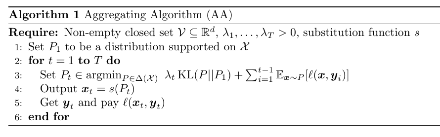
Equipped with this definition, we can introduce the Aggregating Algorithm in Algorithm 1. Its regret guarantee is the following one.
Theorem 5. Assume
to be
, and
for all
Moreover, we also have
![\displaystyle \sum_{t=1}^T \ell( {\boldsymbol x}_t, y_t) \leq \mathop{\mathbb E}_{{\boldsymbol x} \sim Q}\left[\sum_{t=1}^T \ell({\boldsymbol x},{\boldsymbol y}_t)\right] + \lambda_T \text{KL}(Q||P_1), \quad \forall Q \in \Delta(\mathcal{X})~.](https://s0.wp.com/latex.php?latex=%5Cdisplaystyle+%5Csum_%7Bt%3D1%7D%5ET+%5Cell%28+%7B%5Cboldsymbol+x%7D_t%2C+y_t%29+%5Cleq+%5Cmathop%7B%5Cmathbb+E%7D_%7B%7B%5Cboldsymbol+x%7D+%5Csim+Q%7D%5Cleft%5B%5Csum_%7Bt%3D1%7D%5ET+%5Cell%28%7B%5Cboldsymbol+x%7D%2C%7B%5Cboldsymbol+y%7D_t%29%5Cright%5D+%2B+%5Clambda_T+%5Ctext%7BKL%7D%28Q%7C%7CP_1%29%2C+%5Cquad+%5Cforall+Q+%5Cin+%5CDelta%28%5Cmathcal%7BX%7D%29%7E.+&bg=ffffff&fg=000000&s=0&c=20201002)
![\displaystyle \sum_{t=1}^T \ell( {\boldsymbol x}_t,{\boldsymbol y}_t) \leq -\lambda_T \ln \mathop{\mathbb E}_{{\boldsymbol x} \sim P_1}\left[ \exp\left(-\frac{1}{\lambda_T} \sum_{t=1}^T \ell({\boldsymbol x},{\boldsymbol y}_t)\right)\right]~.](https://s0.wp.com/latex.php?latex=%5Cdisplaystyle+%5Csum_%7Bt%3D1%7D%5ET+%5Cell%28+%7B%5Cboldsymbol+x%7D_t%2C%7B%5Cboldsymbol+y%7D_t%29+%5Cleq+-%5Clambda_T+%5Cln+%5Cmathop%7B%5Cmathbb+E%7D_%7B%7B%5Cboldsymbol+x%7D+%5Csim+P_1%7D%5Cleft%5B+%5Cexp%5Cleft%28-%5Cfrac%7B1%7D%7B%5Clambda_T%7D+%5Csum_%7Bt%3D1%7D%5ET+%5Cell%28%7B%5Cboldsymbol+x%7D%2C%7B%5Cboldsymbol+y%7D_t%29%5Cright%29%5Cright%5D%7E.+&bg=ffffff&fg=000000&s=0&c=20201002)
As we did for WAA last time, under additional assumptions we can also give a regret bound with respect to a deterministic competitor.
Theorem 6. Let
a non-empty closed convex set in
and
, where
is an arbitrary norm. Let
and assume that
is
-Lipschitz w.r.t.
such that
satisfies

Proof: We start from the second bound in Theorem 5. Fix ![{\theta \in [0,1]}](https://s0.wp.com/latex.php?latex=%7B%5Ctheta+%5Cin+%5B0%2C1%5D%7D&bg=ffffff&fg=000000&s=0&c=20201002)


![\displaystyle \begin{aligned} \mathop{\mathbb E}_{{\boldsymbol x} \sim P_1} \left[\exp\left(-\frac{1}{\lambda_T} \sum_{t=1}^T \ell({\boldsymbol x}, {\boldsymbol y}_t)\right)\right] &\geq (1-\theta)^d \mathop{\mathbb E}_{{\boldsymbol x} \sim P'_1} \left[\exp\left(-\frac{1}{\lambda_T} \sum_{t=1}^T \ell({\boldsymbol x},{\boldsymbol y}_t)\right)\right] \\ &= (1-\theta)^d \mathop{\mathbb E}_{{\boldsymbol x} \sim P_1} \left[\exp\left(-\frac{1}{\lambda_T} \sum_{t=1}^T\ell(\theta {\boldsymbol u} + (1-\theta){\boldsymbol x},{\boldsymbol y}_t)\right)\right] \\ &= (1-\theta)^d \mathop{\mathbb E}_{{\boldsymbol x} \sim P_1} \left[\exp\left(-\frac{1}{\lambda_T} \sum_{t=1}^T\ell((1-\theta)({\boldsymbol x}-{\boldsymbol u})+{\boldsymbol u},{\boldsymbol y}_t )\right)\right] \\ &\geq (1-\theta)^d \mathop{\mathbb E}_{{\boldsymbol x} \sim P_1} \left[\exp\left(-\frac{1}{\lambda_T} \sum_{t=1}^T\left(\ell({\boldsymbol u},{\boldsymbol y}_t ) + L_t (1-\theta)\|{\boldsymbol x}-{\boldsymbol u}\|\right)\right)\right] \\ &\geq (1-\theta)^d \mathop{\mathbb E}_{{\boldsymbol x} \sim P_1} \left[\exp\left(-\frac{1}{\lambda_T} \sum_{t=1}^T \left(\ell({\boldsymbol u},{\boldsymbol y}_t ) + L_t (1-\theta) D\right)\right)\right] \\ &= (1-\theta)^d \exp\left(-\frac{1}{\lambda_T} \sum_{t=1}^T \ell({\boldsymbol u},{\boldsymbol y}_t )\right) \exp\left(-\frac{1}{\lambda_T} \sum_{t=1}^T L_t (1-\theta)D\right)~. \end{aligned}](https://s0.wp.com/latex.php?latex=%5Cdisplaystyle+%5Cbegin%7Baligned%7D+%5Cmathop%7B%5Cmathbb+E%7D_%7B%7B%5Cboldsymbol+x%7D+%5Csim+P_1%7D+%5Cleft%5B%5Cexp%5Cleft%28-%5Cfrac%7B1%7D%7B%5Clambda_T%7D+%5Csum_%7Bt%3D1%7D%5ET+%5Cell%28%7B%5Cboldsymbol+x%7D%2C+%7B%5Cboldsymbol+y%7D_t%29%5Cright%29%5Cright%5D+%26%5Cgeq+%281-%5Ctheta%29%5Ed+%5Cmathop%7B%5Cmathbb+E%7D_%7B%7B%5Cboldsymbol+x%7D+%5Csim+P%27_1%7D+%5Cleft%5B%5Cexp%5Cleft%28-%5Cfrac%7B1%7D%7B%5Clambda_T%7D+%5Csum_%7Bt%3D1%7D%5ET+%5Cell%28%7B%5Cboldsymbol+x%7D%2C%7B%5Cboldsymbol+y%7D_t%29%5Cright%29%5Cright%5D+%5C%5C+%26%3D+%281-%5Ctheta%29%5Ed+%5Cmathop%7B%5Cmathbb+E%7D_%7B%7B%5Cboldsymbol+x%7D+%5Csim+P_1%7D+%5Cleft%5B%5Cexp%5Cleft%28-%5Cfrac%7B1%7D%7B%5Clambda_T%7D+%5Csum_%7Bt%3D1%7D%5ET%5Cell%28%5Ctheta+%7B%5Cboldsymbol+u%7D+%2B+%281-%5Ctheta%29%7B%5Cboldsymbol+x%7D%2C%7B%5Cboldsymbol+y%7D_t%29%5Cright%29%5Cright%5D+%5C%5C+%26%3D+%281-%5Ctheta%29%5Ed+%5Cmathop%7B%5Cmathbb+E%7D_%7B%7B%5Cboldsymbol+x%7D+%5Csim+P_1%7D+%5Cleft%5B%5Cexp%5Cleft%28-%5Cfrac%7B1%7D%7B%5Clambda_T%7D+%5Csum_%7Bt%3D1%7D%5ET%5Cell%28%281-%5Ctheta%29%28%7B%5Cboldsymbol+x%7D-%7B%5Cboldsymbol+u%7D%29%2B%7B%5Cboldsymbol+u%7D%2C%7B%5Cboldsymbol+y%7D_t+%29%5Cright%29%5Cright%5D+%5C%5C+%26%5Cgeq+%281-%5Ctheta%29%5Ed+%5Cmathop%7B%5Cmathbb+E%7D_%7B%7B%5Cboldsymbol+x%7D+%5Csim+P_1%7D+%5Cleft%5B%5Cexp%5Cleft%28-%5Cfrac%7B1%7D%7B%5Clambda_T%7D+%5Csum_%7Bt%3D1%7D%5ET%5Cleft%28%5Cell%28%7B%5Cboldsymbol+u%7D%2C%7B%5Cboldsymbol+y%7D_t+%29+%2B+L_t+%281-%5Ctheta%29%5C%7C%7B%5Cboldsymbol+x%7D-%7B%5Cboldsymbol+u%7D%5C%7C%5Cright%29%5Cright%29%5Cright%5D+%5C%5C+%26%5Cgeq+%281-%5Ctheta%29%5Ed+%5Cmathop%7B%5Cmathbb+E%7D_%7B%7B%5Cboldsymbol+x%7D+%5Csim+P_1%7D+%5Cleft%5B%5Cexp%5Cleft%28-%5Cfrac%7B1%7D%7B%5Clambda_T%7D+%5Csum_%7Bt%3D1%7D%5ET+%5Cleft%28%5Cell%28%7B%5Cboldsymbol+u%7D%2C%7B%5Cboldsymbol+y%7D_t+%29+%2B+L_t+%281-%5Ctheta%29+D%5Cright%29%5Cright%29%5Cright%5D+%5C%5C+%26%3D+%281-%5Ctheta%29%5Ed+%5Cexp%5Cleft%28-%5Cfrac%7B1%7D%7B%5Clambda_T%7D+%5Csum_%7Bt%3D1%7D%5ET+%5Cell%28%7B%5Cboldsymbol+u%7D%2C%7B%5Cboldsymbol+y%7D_t+%29%5Cright%29+%5Cexp%5Cleft%28-%5Cfrac%7B1%7D%7B%5Clambda_T%7D+%5Csum_%7Bt%3D1%7D%5ET+L_t+%281-%5Ctheta%29D%5Cright%29%7E.+%5Cend%7Baligned%7D&bg=ffffff&fg=000000&s=0&c=20201002)
Putting all together, we have

Now, we set 


2. Example of AA: Online Multiclass Logistic Regression
In this section, we show an application of AA showing how to obtain logarithmic regret for online multiclass logistic regression. In this problem, in each round we receive a covariate 


We could use a linear classifier, 


Here, we show that we can prove a logarithmic bound that depends only logarithmically on
Here, we will proceed a little bit differently than in the standard AA algorithm because we will use two loss functions, 

![\displaystyle \frac{1}{\alpha}\ln \mathop{\mathbb E}_{{\boldsymbol x} \sim P} [\exp(-\alpha \ell_t({\boldsymbol x}, y))] + \hat{\ell}\left(s_t(P), y\right) \leq 0, \quad \forall P \in \Delta(\mathcal{X}), {\boldsymbol y} \in \mathcal{Y}~.](https://s0.wp.com/latex.php?latex=%5Cdisplaystyle+%5Cfrac%7B1%7D%7B%5Calpha%7D%5Cln+%5Cmathop%7B%5Cmathbb+E%7D_%7B%7B%5Cboldsymbol+x%7D+%5Csim+P%7D+%5B%5Cexp%28-%5Calpha+%5Cell_t%28%7B%5Cboldsymbol+x%7D%2C+y%29%29%5D+%2B+%5Chat%7B%5Cell%7D%5Cleft%28s_t%28P%29%2C+y%5Cright%29+%5Cleq+0%2C+%5Cquad+%5Cforall+P+%5Cin+%5CDelta%28%5Cmathcal%7BX%7D%29%2C+%7B%5Cboldsymbol+y%7D+%5Cin+%5Cmathcal%7BY%7D%7E.+&bg=ffffff&fg=000000&s=0&c=20201002)
It is easy to see that Theorem 5 extends to this case:
![\displaystyle \sum_{t=1}^T \hat{\ell}( {\boldsymbol x}_t,{\boldsymbol y}_t) \leq -\lambda_T \ln \mathop{\mathbb E}_{{\boldsymbol x} \sim P_1}\left[ \exp\left(-\frac{1}{\lambda_T} \sum_{t=1}^T \ell_t({\boldsymbol x},{\boldsymbol y}_t)\right)\right]~.](https://s0.wp.com/latex.php?latex=%5Cdisplaystyle+%5Csum_%7Bt%3D1%7D%5ET+%5Chat%7B%5Cell%7D%28+%7B%5Cboldsymbol+x%7D_t%2C%7B%5Cboldsymbol+y%7D_t%29+%5Cleq+-%5Clambda_T+%5Cln+%5Cmathop%7B%5Cmathbb+E%7D_%7B%7B%5Cboldsymbol+x%7D+%5Csim+P_1%7D%5Cleft%5B+%5Cexp%5Cleft%28-%5Cfrac%7B1%7D%7B%5Clambda_T%7D+%5Csum_%7Bt%3D1%7D%5ET+%5Cell_t%28%7B%5Cboldsymbol+x%7D%2C%7B%5Cboldsymbol+y%7D_t%29%5Cright%29%5Cright%5D%7E.+&bg=ffffff&fg=000000&s=0&c=20201002)
Similarly, we have that if 

In particular, from Proposition 3, we will define 
![{s_t(\pi) = \ln \mathop{\mathbb E}_{{\boldsymbol X}\sim\pi}[\sigma({\boldsymbol X}^\top {\boldsymbol z}_t)]}](https://s0.wp.com/latex.php?latex=%7Bs_t%28%5Cpi%29+%3D+%5Cln+%5Cmathop%7B%5Cmathbb+E%7D_%7B%7B%5Cboldsymbol+X%7D%5Csim%5Cpi%7D%5B%5Csigma%28%7B%5Cboldsymbol+X%7D%5E%5Ctop+%7B%5Cboldsymbol+z%7D_t%29%5D%7D&bg=ffffff&fg=000000&s=0&c=20201002)

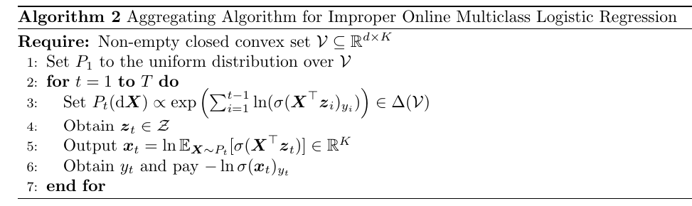
Theorem 7. Assume that
for all
and
. Then, Algorithm 2 satisfies

Proof: We have that
![\displaystyle \frac{\partial \hat{\ell}({\boldsymbol x},y)}{\partial x_j} = \sigma({\boldsymbol x})_j-\boldsymbol{1}[y=j]~.](https://s0.wp.com/latex.php?latex=%5Cdisplaystyle+%5Cfrac%7B%5Cpartial+%5Chat%7B%5Cell%7D%28%7B%5Cboldsymbol+x%7D%2Cy%29%7D%7B%5Cpartial+x_j%7D+%3D+%5Csigma%28%7B%5Cboldsymbol+x%7D%29_j-%5Cboldsymbol%7B1%7D%5By%3Dj%5D%7E.+&bg=ffffff&fg=000000&s=0&c=20201002)
Defining 


6. History Bits
The AA was introduced in Vovk (1990) (see also Vovk (1998, Appendix A) for an easier description of the algorithm).
The observation that the AA also works for infinite sets of experts was made by Freund (1996), Freund (2003).
The concept of mixability is introduced in Vovk (2001). Proposition 2 is in the proof of Vovk (1998, Lemma 9).
The mixability of the logistic loss, Proposition 3, and the content of Section 2 are from Foster et al. (2018). Theorem 6 is a generalization of a similar one for the logistic loss from Foster et al. (2018).
Acknowledgments
Thanks to Wei-Cheng Lee for feedback on a prelimary version of this post and to Gemini 2.5 and ChatGPT5 for checking all the proofs.
