Parameter-free Online Learning I: Coin-Betting and 1-d OCO

This post is part of the lecture notes of my class “Introduction to Online Learning” at Boston University, Fall 2019.

You can find all the lectures I published here.

In the previous classes, we have shown that Online Mirror Descent (OMD) and Follow-The-Regularized-Leader (FTRL) achieves a regret of ${O(\sqrt{T})}$ for convex Lipschitz losses. We have also shown that for bounded domains these bounds are optimal up to constant multiplicative factors. However, in the unbounded case the bounds we get are suboptimal w.r.t. the dependency on the competitor. More in particular, let’s consider an example with Online Subgradient Descent with ${V={\mathbb R}^d}$ over ${1}$ -Lipschitz losses and learning rate ${\eta=\frac{\alpha}{\sqrt{T}}}$ . We get the following regret guarantee

$\displaystyle \text{Regret}_T({\boldsymbol u}) = \sum_{t=1}^T \ell_t({\boldsymbol x}_t) - \sum_{t=1}^T \ell_t({\boldsymbol u}) \leq \frac{\|{\boldsymbol u}\|_2^2}{2\eta} + \frac{\eta T}{2} = \frac{1}{2}\sqrt{T} \left(\frac{\|{\boldsymbol u}\|_2^2}{\alpha}+\alpha\right)~.$

So, in order to get the best possible guarantee, we should know ${\|{\boldsymbol u}\|_2}$ and set ${\alpha=\|{\boldsymbol u}\|_2}$ . As we said, this strategy does not work for a couple of reasons: i) we don’t know ${\|{\boldsymbol u}\|_2}$ ii) if we guessed any value of ${\|{\boldsymbol u}\|_2}$ the adversary could easily change the losses to make that value completely wrong.

Far from being a technicality, this is an important issue as shown in the next example.

Example 1 Consider that we want to use OSD with online-to-batch conversion to minimize a function that is 1-Lipschitz. The convergence rate will be ${O((\tfrac{\|{\boldsymbol u}^\star\|_2^2}{\alpha}+\alpha)\sqrt{T})}$ using a learning rate of ${\eta=\frac{\alpha}{\sqrt{T}}}$ . Consider the case that ${\|{\boldsymbol u}^\star\|_2=100}$ , specifying ${\alpha=1}$ will result in a convergence rate 100 times slower that specifying the optimal choice in hindsight ${\alpha=100}$ . Note that this is a real effect not an artifact of the proof. Indeed,it is intuitive that the optimal learning rate should be proportional to the distance between the initial point that algorithm picks and the optimal solution.

If we could tune the learning rate in the optimal way, we would get a regret of

$\displaystyle \text{Regret}_T({\boldsymbol u}) \leq \|{\boldsymbol u}\|_2 \sqrt{T}~.$

However, this is also impossible, because we proved a lower bound that says that the regret must be ${\Omega(\|{\boldsymbol u}\|_2\sqrt{T \ln \left(\|{\boldsymbol u}\|_2+1\right)})}$ .

In the following, we will show that it is possible to reduce any Online Convex Optimization (OCO) game to betting on a non-stochastic coin. This will allow us to use a radically different way to design OCO algorithms that will enjoy the optimal regret and will not require any parameter (e.g. learning rates, regularization weights) to be tuned. We call these kind of algorithms parameter-free.

1. Coin-Betting Game

Imagine the following repeated game:

Set the initial Wealth to ${\epsilon}$ : ${\text{Wealth}_0=\epsilon}$ .
In each round
- You bet ${|x_t|}$ money on side of the coin equal to ${\rm sign(x_t)}$ ; you cannot bet more money than what you currently have.
- The adversary reveals the outcome of the coin ${c_t \in \{-1, 1\}}$ .
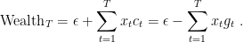
- You gain money ${x_t c_t }$ , that is ${\text{Wealth}_t=\text{Wealth}_{t-1}+c_t x_t = \epsilon + \sum_{i=1}^{t} c_i x_i}$ .

Given that we cannot borrow money, we can codify the bets ${x_t}$ as ${\beta_t \text{Wealth}_{t-1}}$ , with ${\beta_t \in [-1,1]}$ . So, ${|\beta_t|}$ is the fraction of money to bet and ${\rm sign(\beta_t)}$ the side of the coin on which we bet.

The aim of the game is to make as much money as possible. As usual, given the adversarial nature of the game, we cannot hope to always win money. Instead, we try to gain as much money as the strategy that bets a fixed amount of money ${\beta^\star \in [-1, 1]}$ for the entire game.

Note that

$\displaystyle \text{Wealth}_t = \text{Wealth}_{t-1} + c_t x_t =\text{Wealth}_{t-1} + \beta_t \text{Wealth}_{t-1} c_t = \text{Wealth}_{t-1} (1 + \beta_t c_t) = \epsilon\prod_{i=1}^{t-1} (1+ \beta_i c_i)~.$

So, given the multiplicative nature of the wealth, it is also useful to take the logarithm of the ratio of the wealth of the algorithm and wealth of the optimal betting fraction. Hence, we want to minimize the following regret

$\displaystyle \begin{aligned} \ln \max_{\beta \in [-1,1]} \epsilon \prod_{t=1}^T (1+\beta c_t) - \ln \text{Wealth}_T &= \ln \max_{\beta \in [-1,1]} \epsilon \prod_{t=1}^T (1+\beta c_t) - \ln \left(\epsilon \prod_{t=1}^T (1+\beta_t c_t)\right) \\ &= \max_{\beta \in [-1,1]} \sum_{t=1}^T \ln(1+\beta c_t) - \sum_{t=1}^T \ln(1+\beta_t c_t)~. \end{aligned}$

In words, this is nothing else than the regret of an OCO game where the losses are ${\ell_t(x)=-\ln(1+x c_t)}$ and ${V=[-1,1]}$ . We can also extend a bit the formulation allowing “continuous coins”, where ${c_t \in [-1, 1]}$ rather than in ${\{-1, 1\}}$ .

Remark 1 Note that the constraint to bet a fraction between ${-1}$ and ${1}$ is not strictly necessary. We could allow the algorithm to bet more money that what it currently has, lending it some money in each round. However, the restriction makes the analysis easier because it allows the transfomation above into an OCO problem, using the non-negativity of ${1+\beta_t c_t}$ .

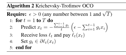
We could just use OMD or FTRL, taking special care of the non-Lipschitzness of the functions, but it turns out that there exists a better strategy specifically for this problem. There exists a very simple strategy to solve the coin-betting game above, that is called Krichevsky-Trofimov (KT) bettor. It simply says that on each time step ${t}$ you bet ${\beta_t=\frac{\sum_{i=1}^{t-1} c_i}{t}}$ . So, the algorithm is the following one.

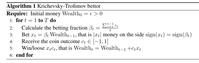
For it, we can prove the following theorem.

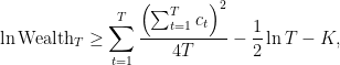
Theorem 1 (Cesa-Bianchi, N. and Lugosi, G. , 2006, Theorem 9.4) Let ${c_t \in \{-1, 1\}}$ for ${t=1, \dots, T}$ . Then, the KT bettor in Algorithm 1 guarantees

$\displaystyle \ln \text{Wealth}_T \geq \ln \max_{\beta \in [-1,1]} \prod_{t=1}^T (1+\beta c_t) - \frac{1}{2} \ln T - K,$

where ${K}$ is a universal constant.

Note that if the outcomes of the coin are skewed towards one side, the optimal betting fraction will gain an exponential amount of money, as proved in the next Lemma.

Lemma 2 Let ${g_t\in \{-1,1\}, t=1,\dots,T}$ . Then, we have

$\displaystyle \max_{\beta \in [-1,1]} \exp\left( \sum_{t=1}^T \ln (1-\beta g_t) \right) \geq \exp\left(\sum_{t=1}^T \frac{\left(\sum_{t=1}^T g_t\right)^2}{4T}\right)~.$

Proof:

$\displaystyle \begin{aligned} \max_{\beta \in [-1,1]} \exp\left( \sum_{t=1}^T \ln (1-\beta g_t) \right) &\geq \max_{\beta \in [-1/2,1/2]} \exp\left( \sum_{t=1}^T \ln (1-\beta g_t) \right) \geq \max_{\beta \in [-1/2,1/2]} \exp\left( \beta \sum_{t=1}^T g_t - \beta^2 \sum_{t=1}^T g_t^2 \right) \\ &= \max_{\beta \in [-1/2,1/2]} \exp\left( \beta \sum_{t=1}^T g_t - \beta^2 T \right) = \exp\left( \frac{\left(\sum_{t=1}^T g_t\right)^2}{4T} \right)~. \end{aligned}$

where we used the elementary inequality ${\ln(1+x)\geq x - x^2}$ for ${x \in [-1/2, 1/2]}$ . $\Box$

Hence, KT guarantees an exponential amount of money, paying only a ${\sqrt{T}}$ penalty. It is possible to prove that the guarantee above for the KT algorithm is optimal to constant additive factors. Moreover, observe that the KT strategy does not require any parameter to be set: no learning rates, nor regularizer. That is, KT is parameter-free.

Also, we can extend the guarantee of the KT algorithm to the case in which the coin are “continuous”, that is ${c_t \in [-1,1]}$ . We have the following Theorem.

Theorem 3 (Orabona, F. and Pal, D., 2016, Lemma 14) Let ${c_t \in [-1, 1]}$ for ${t=1, \dots, T}$ . Then, the KT bettor in Algorithm 1 guarantees

$\displaystyle \ln \text{Wealth}_T\geq \sum_{t=1}^T \frac{\left(\sum_{t=1}^T c_t\right)^2}{4T} - \frac{1}{2} \ln T - K,$

where ${K}$ is a universal constant.

So, we have introduced the coin-betting game, extended it to continuous coins and presented a simple and optimal parameter-free strategy. In the next Section, we show how to use the KT bettor as a parameter-free 1-d OCO algorithm!

2. Parameter-free 1d OCO through Coin-Betting

So, Theorem 1 tells us that we can win almost as much money as a strategy betting the optimal fixed fraction of money at each step. We only pay a logarithmic price in the log wealth, that corresponds to a ${\frac{1}{\sqrt{T}}}$ term in the actual wealth.

Now, let’s see why this problem is interesting in OCO. It turns out that solving the coin-betting game is equivalent to solving a 1-dimensional unconstrained online linear optimization problem. That is, a coin-betting algorithm is equivalent to design an online learning algorithm that produces a sequences of ${x_t\in {\mathbb R}}$ that minimize the 1-dimensional regret with linear losses:

$\displaystyle \text{Regret}_T(u):=\sum_{t=1}^T g_t x_t - \sum_{t=1}^T g_t u,$

where the ${g_t}$ are adversarial and bounded. Without loss of generality, we will assume ${g_t \in [-1,1]}$ . Also, remembering that OCO games can be reduced to Online Linear Optimization (OLO) games, such reduction would effectively reduces OCO to coin-betting! Moreover, through online-to-batch conversion, any stochastic 1-d problem could be reduced to a coin-betting game! The key theorem that allows the conversion between OLO and coin-betting is the following one.

Theorem 4 Let ${\phi:{\mathbb R}^d \rightarrow (-\infty,+\infty]}$ be a proper closed convex function and let ${\phi^\star:{\mathbb R}^d \rightarrow (-\infty,+\infty]}$ be its Fenchel conjugate. An algorithm that generates ${{\boldsymbol x}_1, {\boldsymbol x}_2, \dots, {\boldsymbol x}_T \in {\mathbb R}^d}$ guarantees

$\displaystyle \forall {\boldsymbol g}_1,\dots,{\boldsymbol g}_T \in {\mathbb R}^d, \quad \epsilon-\sum_{t=1}^T \langle {\boldsymbol g}_t, {\boldsymbol x}_t \rangle \ge \phi\left( -\sum_{t=1}^T {\boldsymbol g}_t \right)$

where ${\epsilon \in {\mathbb R}}$ , if and only if it guarantees

$\displaystyle \forall {\boldsymbol u} \in {\mathbb R}^d, \quad \underbrace{\sum_{t=1}^T \langle {\boldsymbol g}_t, {\boldsymbol x}_t - {\boldsymbol u}\rangle}_{\text{Regret}_T({\boldsymbol u})} \le \phi^\star({\boldsymbol u})+\epsilon~.$

Proof: Let’s prove the left to right implication.

$\displaystyle \begin{aligned} \text{Regret}_T({\boldsymbol u}) &= \sum_{t=1}^T \langle {\boldsymbol g}_t, {\boldsymbol x}_t - {\boldsymbol u}\rangle \le -\sum_{t=1}^T \langle {\boldsymbol g}_t, {\boldsymbol u} \rangle - \phi\left(-\sum_{t=1}^T {\boldsymbol g}_t\right) + \epsilon\\ &\leq \sup_{{\boldsymbol \theta} \in {\mathbb R}^d} \ \langle {\boldsymbol \theta}, {\boldsymbol u} \rangle - \phi\left( {\boldsymbol \theta} \right) +\epsilon = \phi^\star\left({\boldsymbol u}\right)+\epsilon~. \end{aligned}$

For the other implication, we have

$\displaystyle \begin{aligned} -\sum_{t=1}^T \langle {\boldsymbol g}_t, {\boldsymbol x}_t \rangle &= -\sum_{t=1}^T \langle {\boldsymbol g}_t, {\boldsymbol u} \rangle - \sum_{t=1}^T \langle {\boldsymbol g}_t, {\boldsymbol x}_t - {\boldsymbol u} \rangle \\ &= \sup_{{\boldsymbol u} \in {\mathbb R}^d} \ -\sum_{t=1}^T \langle {\boldsymbol g}_t, {\boldsymbol u} \rangle - \sum_{t=1}^T \langle {\boldsymbol g}_t, {\boldsymbol x}_t - {\boldsymbol u} \rangle \\ &\ge \sup_{{\boldsymbol u} \in {\mathbb R}^d} \ -\sum_{t=1}^T \langle {\boldsymbol g}_t, {\boldsymbol u} \rangle - \phi^\star\left({\boldsymbol u}\right) - \epsilon = \phi\left(-\sum_{t=1}^T {\boldsymbol g}_t\right) - \epsilon~. \end{aligned}$

$\Box$

To make sense of the above theorem, assume that we are considering a 1-d problem and ${g_t \in [-1,1]}$ . Then, guaranteeing a lower bound to

$\displaystyle \epsilon-\sum_{t=1}^T \langle {\boldsymbol g}_t, {\boldsymbol x}_t \rangle$

can be done through a betting strategy that bets ${x_t}$ money on the coins ${c_t=-g_t}$ . So, the theorem implies that proving a reward lower bound for the wealth in a coin-betting game implies a regret upper bound for the corresponding 1-dimensional OLO game. However, proving a reward lower bound is easier because it doesn’t depend on the competitor ${{\boldsymbol u}}$ . Indeed, not knowing the norm of the competitor is exactly the reason why tuning the learning rates in OMD is hard!

This consideration immediately gives us the conversion between 1-d OLO and coin-betting: the outcome of the coin is the negative of the subgradient of the losses on the current prediction. Indeed, setting ${c_t=-g_t}$ , we have that a coin-betting algorithm that bets ${x_t}$ would give us

$\displaystyle \text{Wealth}_{T} =\epsilon + \sum_{t=1}^T x_t c_t =\epsilon - \sum_{t=1}^T x_t g_t ~.$

So, a lower bound on the wealth corresponds to a lower bound that can be used in Theorem 3. To obtain a regret guarantee, we only need to calculate the Fenchel conjugate of the reward function, assuming it can be expressed as a function of ${\sum_{t=1}^T c_t}$ .

The last step is to reduce 1-d OCO to 1-d OLO. But, this is an easy step that we have done many times. Indeed, we have

$\displaystyle \text{Regret}_T(u)=\sum_{t=1}^T \ell_t(x_t) -\sum_{t=1}^T \ell_t(u) \leq \sum_{t=1}^T x_t g_t - \sum_{t=1}^T g_t u,$

where ${g_t \in \partial \ell_t(x_t)}$ .

So, to summarize, the Fenchel conjugate of the wealth lower bound for the coin-betting game becomes the regret guarantee for the OCO game. In the next section, we specialize all these considerations to the KT algorithm.

3. KT as a 1d Online Convex Optimization Algorithm

Here, we want to use the considerations in the above section to use KT as a parameter-free 1-d OCO algorithm. First, let’s see what such algorithm looks like. KT bets ${x_t=\beta_t \text{Wealth}_{t-1}}$ , starting with ${\epsilon}$ money. Now, set ${c_t=-g_t}$ where ${g_t \in \partial \ell_t(x_t)}$ and assume the losses ${\ell_t}$ ${1}$ -Lipschitz. So, we get

$\displaystyle x_t = -\frac{\sum_{i=1}^{t-1} g_i}{t} \left(\epsilon - \sum_{i=1}^{t-1} g_i x_i\right)~.$

The pseudo-code is in Algorithm 3.

kt_oco

Let’s now see what kind of regret we get. From Theorem 3 and Lemma 2, we have that the KT bettor guarantees the following lower bound on the wealth when used with ${c_t=-g_t}$ :

$\displaystyle \epsilon-\sum_{t=1}^T x_t g_t \geq \frac{\epsilon}{K\sqrt{T}}\exp\left(\frac{(\sum_{t=1}^T g_t)^2}{4T}\right)~.$

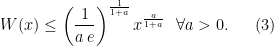
So, we found the function ${\phi}$ , we just need ${\phi^\star}$ or an upper bound to it, that can be found with the following Lemma.

Lemma 5 Define ${f(x)= \beta \exp\frac{x^2}{2 \alpha}}$ , for ${\alpha,\beta>0}$ , ${x\geq0}$ . Then

$\displaystyle \begin{aligned} f^\star(y) &=|y| \sqrt{\alpha W\left(\frac{\alpha y^2}{\beta^2}\right)} - \beta \exp\left(\frac{W\left(\frac{\alpha y^2}{\beta^2}\right)}{2}\right) \leq |y| \sqrt{\alpha W\left(\frac{\alpha y^2}{\beta^2}\right)} - \beta \leq |y| \sqrt{\alpha \ln\left(1+\frac{\alpha y^2}{\beta^2}\right)} - \beta~. \end{aligned}$

where ${W(x)}$ is the Lambert function, i.e. ${W:{\mathbb R}_+\rightarrow {\mathbb R}_+}$ defined as to satisfy ${x=W(x) \exp(W(x))}$ .

Proof: From the definition of Fenchel dual, we have

$\displaystyle \begin{aligned} f^\star(y)= \max_{x} \ x\, y - f(x) = \max_{x} \ x\, y - \beta \exp\frac{x^2}{2 \alpha} \leq x^\star\,y -\beta, \end{aligned}$

where ${x^\star= \mathop{\mathrm{argmax}}_{x} x\, y - f(x)}$ . We now use the fact that ${x^\star}$ satisfies ${y = f'(x^\star)}$ , to have ${x^\star=\rm sign(y)\sqrt{\alpha W\left(\frac{\alpha y^2}{\beta^2}\right)}}$ , where ${W(\cdot)}$ is the Lambert function. Using Lemma 5 in the Appendix, we obtain the stated bound. $\Box$

So, the regret guarantee of KT used a 1d OLO algorithm is upper bounded by

$\displaystyle \text{Regret}_T(u) =\sum_{t=1}^T \ell_t(x_t) - \sum_{t=1}^T \ell_t(u) \leq |u| \sqrt{4 T \ln \left(\frac{\sqrt{2} |u| K T }{\epsilon}+1\right)} + \epsilon, \ \forall u \in {\mathbb R},$

where the only assumption was that the first derivatives (or sub-derivatives) of ${\ell_t}$ are bounded in absolute value by 1. Also, it is important to note that any setting of ${\epsilon}$ in ${[1,\sqrt{T}]}$ would not change the asymptotic rate.

To better appreciate this regret, compare this bound to the one of OMD with learning rate ${\eta=\frac{\alpha}{\sqrt{T}}}$ :

$\displaystyle \text{Regret}_T(u) =\sum_{t=1}^T \ell_t(x_t) -\sum_{t=1}^T \ell_t(u) \leq \frac{1}{2}\left(\frac{u^2}{\alpha}+\alpha\right)\sqrt{T}, \ \forall u \in {\mathbb R}~.$

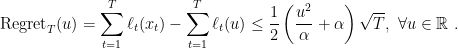
Hence, the coin-betting approach allows to get almost the optimal bound, without having to guess the correct learning rate! The price that we pay for this parameter-freeness is the log factor, that is optimal from our lower bound.

It is interesting also to look at what the algorithm would do on an easy problem, where ${\ell_t(x)=|x-10|}$ . In Figure 3, we show the different predictions that the KT algorithm and online subgradient descent (OSD) would do. Note how the convergence rate of OSD critically depends on the learning rate: too big will not give convergence and too small will make slow down the convergence. On the other hand, KT will go exponentially fast towards the minimum and then it will automatically backtrack. This exponential growth effectively works like a line search procedure that allows to get the optimal regret without tuning learning rates. Later in the iterations, KT will oscillate around the minimum, automatically shrinking its steps, without any parameter to tune. Of course, this is a simplified example. In a truly OCO game, the losses are different at each time step and the intuition behind the algorithm becomes more difficult. Yet, the optimality of the regret assures us that the KT strategy is the right strategy.

comparison_kt — Behaviour of KT (left) and online gradient descent with various learning rates and same number of steps (right) when ${\ell_t(x)=|x-10|}$ .

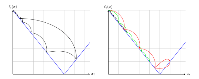Next time, we will see that we can also reduce OCO in ${{\mathbb R}^d}$ and learning with experts to coin-betting games.

4. History Bits

The keyword “parameter-free” has been introduced in (Chaudhuri, K. and Freund, Y. and Hsu, D. J., 2009) for a similar strategy for the learning with expert problem. It is now used as an umbrella term for all online algorithms that guarantee the optimal regret uniformly over the competitor class. The first algorithm for 1-d parameter-free OCO is from (M. Streeter and B. McMahan, 2012), but the bound was suboptimal. The algorithm was then extended to Hilbert spaces in (Orabona, F., 2013), still with a suboptimal bound. The optimal bound in Hilbert space was obtained in (McMahan, H. B. and Orabona, F., 2014). The idea of using a coin-betting to do parameter-free OCO was introduced in (Orabona, F. and Pal, D., 2016). The Krichevsky-Trofimov algorithm is from (Krichevsky, R. and Trofimov, V., 1981) and its extension to the “continuous coin” is from (Orabona, F. and Pal, D., 2016). The regret-reward duality relationship was proved for the first time in (McMahan, H. B. and Orabona, F., 2014). Lemma 5 is from (Orabona, F. and Pal, D., 2016).

5. Exercises

Exercise 1 While the original proof of the KT regret bound is difficult, it is possible to obtain a looser bound using the be-the-leader method in FTRL. In particular, it is easy to show a regret of ${O(\ln T)}$ for the log wealth.

6. Appendix

The Lambert function ${W(x):{\mathbb R}_+ \rightarrow {\mathbb R}_+}$ is defined by the equality

$\displaystyle \label{eq:lambert} x=W(x) \exp \left(W(x)\right) \qquad \qquad \text{for } x \ge 0~. \ \ \ \ \ (1)$

The following lemma provides bounds on ${W(x)}$ .

Lemma 5 The Lambert function ${W(x)}$ satisfies

$\displaystyle 0.6321 \log(x+1) \leq W(x) \leq \log(x+1), \ \forall x \ge 0~.$

Proof: The inequalities are satisfied for ${x=0}$ , hence we in the following we assume ${x>0}$ . We first prove the lower bound. From (1) we have

$\displaystyle W(x) = \log\left(\frac{x}{W(x)}\right)~. \label{eq:lm_lambert_1} \ \ \ \ \ (2)$

From this equality, using the elementary inequality ${\ln (x) \leq \frac{a}{e} x^\frac{1}{a}}$ for any ${a>0}$ , we get

$\displaystyle W(x) \leq \frac{1}{a\, e}\left(\frac{x}{W(x)}\right)^a \ \ \forall a>0,$

that is

$\displaystyle \label{eq:lm_lambert_2} W(x) \leq \left(\frac{1}{a\, e}\right)^\frac{1}{1+a} x^\frac{a}{1+a} \ \ \forall a>0. \ \ \ \ \ (3)$

Using (3) in (2), we have

$\displaystyle \begin{aligned} W(x) \geq \log\left(\frac{x}{\left(\frac{1}{a\, e}\right)^\frac{1}{1+a} x^\frac{a}{1+a}}\right) = \frac{1}{1+a}\log\left(a \, e\, x\right) \ \ \forall a>0~. \end{aligned}$

Consider now the function ${g(x)=\frac{x}{x+1} - \frac{b}{\log(1+b) (b+1)} \log(x+1)}$ defined in ${[0,b]}$ where ${b}$ is a positive number that will be decided in the following. This function has a maximum in ${x^*=(1+\frac{1}{b}) \log(1+b)-1}$ , the derivative is positive in ${[0,x^*]}$ and negative in ${[x^*,b]}$ . Hence the minimum is in ${x=0}$ and in ${x=b}$ , where it is equal to ${0}$ . Using the property just proved on ${g}$ , setting ${a=\frac{1}{x}}$ , we have

$\displaystyle \begin{aligned} W(x) \geq \frac{x}{x+1} \geq \frac{b}{\log(1+b) (b+1)} \log(x+1) \ \ \forall x\leq b~. \end{aligned}$

For ${x>b}$ , setting ${a=\frac{x+1}{e x}}$ , we have

$\displaystyle \begin{aligned} W(x) &\geq \frac{e\,x}{(e+1) x + 1} \log(x+1) \geq \frac{e\,b}{(e+1) b + 1} \log(x+1) \ \ \ \ \ (4)\end{aligned}$

Hence, we set ${b}$ such that

$\displaystyle \frac{e\, b}{(e+1)b + 1} = \frac{b}{\log(1+b) (b+1)}$

Numerically, ${b=1.71825...}$ , so

$\displaystyle W(x) \geq 0.6321 \log(x+1)~.$

For the upper bound, we use Theorem 2.3 in (Hoorfar, A. and Hassani, M., 2008), that says that

$\displaystyle W(x) \leq \log\frac{x+C}{1+\log(C)}, \quad \forall x> -\frac{1}{e}, \ C>\frac{1}{e}.$

Setting ${C=1}$ , we obtain the stated bound. $\Box$

5 Comments

Pingback: Parameter-free Online Learning II: Reductions – Parameter-free Learning and Optimization Algorithms
bremen79 says:

November 1, 2019 at 11:28 AM

EDIT: Fixed a small bug in the KT guarantee, now the guarantee is split in two theorems one for the “standard” coins and the other one for “continuous” coins.

LikeLike

Pingback: Online Mirror Descent III: Examples and Learning with Expert Advice – Parameter-free Learning and Optimization Algorithms
Frank Lee says:

April 5, 2022 at 5:59 AM

Hi, Francesco. I have the problem with where you get the lower bound of the online sub-gradient descent algorithm is $\Omega(||u||_2\sqrt{T\ln(||u||_2+1)})$ . I guess it is from theorem 5.12 in the book but I’m not sure.

LikeLike

bremen79 says:

April 5, 2022 at 10:05 AM

Hi Frank, the theorem is 5.17 in the latest version of my notes on ArXiv or as a blog post https://parameterfree.com/2019/09/25/lower-bounds-for-online-linear-optimization/.
That said, I am rewriting the lower bound in these days because the stated lower bound holds only for a single vector u, while we want one that holds for any u. I’ll probably put a blog post on it when I have some spare time. In the while, you can find the better lower bound in my 2013 NeurIPS paper (https://francesco.orabona.com/papers/13nips_a_long.pdf).

LikeLike

1. Frank Lee says:
  
  April 6, 2022 at 1:26 AM
  
  Thank you so much, Francesco. Now I know the bound is from theorem 5.17 in the latest version of your excellent notes, but I still have a problem with it. In theorem 5.17, you have $\epsilon(T)$ in the bound, but you don’t have it in the lower bound of online sub-gradient descent. How do you remove it? I also notice that in the bound stated in theorem 5.17, you have $T$ dependency inside of $\ln$ while you don’t have it on the other lower bound. Is it canceled by the $\epsilon(T)$?
  
  Recently, I’ve been reading your ICML tutorial. I have a related question on tutorial slide part 1 page 33 and page 38. On page 33, you stated a decreasing learning rate $\frac{\alpha}{\sqrt{t}}$ will get a bound $O(\frac{1}{\sqrt}(\frac{||x^*-x_1||^2}{\alpha}+\alphaG^2))$ . How do you get it? I know how to derive a bound for a fixed learning rate but have no idea of a decreasing learning rate. I try to use theorem 2.13 to prove it, but in theorem 2.13, we bound the regret using the diameter instead of the distance between the optimal point and the initial point. On page 38, you also state two lower bounds, Is it the same lower bound as theorem 5.17 in the note? If not, what reference could I find the bound?
  
  Last but not least, thank you for pointing out your NeruIPS 2013 paper. I guess the lower bound is from theorem 2. I am looking forward to seeing your new blog post!
  
  LikeLike
  
  1. bremen79 says:
    
    April 13, 2022 at 7:19 PM
    
    For your first question, I am not sure what you mean by epsilon(T) is not in the lower bound of online sub-gradient descent. Maybe upper bound of OGD? If yes, epsilon(T) is there: for u=0, the regret of OGD with eta = O(1/sqrt{T}) is still O(sqrt(T))=epsilon(T).
    Regarding the T in the log, yes it can be cancelled with epsilon(T). However, the correct lower bound has sqrt{T} inside the log, so you can cancel it with epsilon(T)=sqrt{T}. The stated lower bound is correct, but it is for a fixed u. So, it is possible to have log(T ||u||) = constant * log(sqrt{T} ||u||). Hence, this lower bound cannot capture the right dependencies.
    
    For the question on the tutorial, you are right! It should be a fixed learning rate depending on T. However, you can get that rate with FTRL and increasing regularizer, but it is not exactly the same as SGD.
    
    LikeLike