Follow-The-Regularized-Leader II: Applications

This post is part of the lecture notes of my class “Introduction to Online Learning” at Boston University, Fall 2019.

You can find all the lectures I published here.

Last time, we saw that we can use Follow-The-Regularized-Leader (FTRL) on linearized losses:

ftrl_algo_linear2

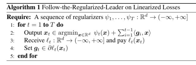
Today, we will show a number of applications of FTRL with linearized losses, some easy ones and some more advanced ones.

As a remainder, the regret upper bound for FTRL for linearized losses that we proved last time for the case that the ${F_t({\boldsymbol x})=\psi({\boldsymbol x})+\sum_{i=1}^{t-1} \ell({\boldsymbol x})}$ is ${\lambda_t}$ -strongly convex w.r.t. ${\|\cdot\|}$ for ${t=1, \dots,T}$ is

$\displaystyle \label{eq:ftrl_bound} \sum_{t=1}^T ( \ell_t({\boldsymbol x}_t) - \ell_t({\boldsymbol u}) ) \leq \psi_{T+1}({\boldsymbol u}) - \min_{{\boldsymbol x}} \ \psi_{1}({\boldsymbol x}) + \sum_{t=1}^T \left(\frac{\|{\boldsymbol g}_t\|_*^2}{2\lambda_t} + \psi_t({\boldsymbol x}_{t+1}) - \psi_{t+1}({\boldsymbol x}_{t+1})\right)~. \ \ \ \ \ (1)$

We also said that we are free to choose ${\psi_{T+1}}$ , so we will often set it to ${\psi_T}$ .

Remark 1 As we said last time, the algorithm is invariant to any positive constant added to the regularizer, hence we can always state the regret guarantee with ${\psi_t({\boldsymbol u})-\min_{{\boldsymbol x}}\psi_t({\boldsymbol x})}$ instead of ${\psi_t}$ . However, for clarity in the following we will instead explicitly choose the regularizer such that their minimum is 0.

1. FTRL with Linearized Losses Can Be Equivalent to OMD

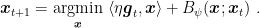
First, we see that even if FTRL and OMD seem very different, in certain cases they are equivalent. For example, consider that case that ${V=X=\mathop{\mathrm{dom}} \psi}$ . The output of OMD is

$\displaystyle {\boldsymbol x}_{t+1} = \mathop{\mathrm{argmin}}_{{\boldsymbol x}} \ \langle \eta {\boldsymbol g}_t, {\boldsymbol x}\rangle + B_\psi({\boldsymbol x};{\boldsymbol x}_t)~.$

Assume that ${{\boldsymbol x}_{t+1} \in \mathop{\mathrm{int}} \mathop{\mathrm{dom}} \psi}$ for all ${t=1, \dots, T}$ . This implies that ${\eta {\boldsymbol g}_t + \nabla \psi({\boldsymbol x}_{t+1}) - \nabla \psi({\boldsymbol x}_t)=\boldsymbol{0}}$ , that is ${ \nabla \psi({\boldsymbol x}_{t+1}) = \nabla \psi({\boldsymbol x}_{t}) -\eta {\boldsymbol g}_t}$ . Assuming ${{\boldsymbol x}_1=\min_{{\boldsymbol x} \in V} \psi({\boldsymbol x})}$ , we have

$\displaystyle \nabla \psi({\boldsymbol x}_{t+1}) = - \eta \sum_{i=1}^t {\boldsymbol g}_i~.$

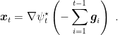
On the other hand, consider FTRL with linearized losses with regularizers ${\psi_t= \frac{1}{\eta} \psi}$ , then

$\displaystyle {\boldsymbol x}_{t+1} = \mathop{\mathrm{argmin}}_{{\boldsymbol x}} \ \frac{1}{\eta} \psi({\boldsymbol x}) + \sum_{i=1}^t \langle {\boldsymbol g}_i, {\boldsymbol x}\rangle = \mathop{\mathrm{argmin}}_{{\boldsymbol x}} \ \psi({\boldsymbol x}) + \eta \sum_{i=1}^t \langle {\boldsymbol g}_i, {\boldsymbol x}\rangle~.$

Assuming that ${{\boldsymbol x}_{t+1} \in \mathop{\mathrm{int}} \mathop{\mathrm{dom}} \psi}$ , this implies that ${\nabla \psi({\boldsymbol x}_{t+1})=-\eta \sum_{i=1}^t {\boldsymbol g}_i}$ . Further, assuming that ${\nabla \psi}$ is invertible, implies that the predictions of FTRL and OMD are the same.

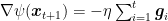
This equivalence immediately gives us some intuition on the role of ${\psi}$ in both algorithm: The same function is inducing the Bregman divergence, that is our similarity measure, and is the regularizer in FTRL. Moreover, the inverse of the growth rate of the regularizers in FTRL takes the role of the learning rate in OMD.

Example 1 Consider ${\psi({\boldsymbol x})=\frac{1}{2}\|{\boldsymbol x}\|_2^2}$ and ${V={\mathbb R}^d}$ , then it satisfies the conditions above to have the predictions of OMD equal to the ones of FTRL.

2. Exponentiated Gradient with FTRL: No Need to know ${T}$

Let’s see an example of an instantiation of FTRL with linearized losses to have the FTRL version of Exponentiated Gradient (EG).

Let ${V=\{{\boldsymbol x} \in {\mathbb R}^d: \|{\boldsymbol x}\|_1=1, x_i\geq0\}}$ and the sequence of loss functions ${\ell_t:V\rightarrow {\mathbb R}}$ be convex and ${L_\infty}$ -Lipschitz w.r.t. the L-infinity norm. Let ${\psi:V\rightarrow {\mathbb R}^d}$ defined as ${\psi({\boldsymbol x})=\sum_{i=1}^d x_i \ln x_i}$ , where ${V=\{{\boldsymbol x} \in {\mathbb R}^d: \|{\boldsymbol x}\|_1=1, x_i\geq0\}}$ and we define ${0\ln0=0}$ . Set ${\psi_t({\boldsymbol x})=\alpha L_\infty \sqrt{t} \psi({\boldsymbol x})}$ , that is ${\alpha L_\infty \sqrt{t}}$ -strongly convex w.r.t. the L1 norm, where ${\alpha>0}$ is a parameter of the algorithm.

Given that the regularizers are strongly convex, we know that

$\displaystyle {\boldsymbol x}_t = \nabla \psi_t^\star \left(-\sum_{i=1}^{t-1} {\boldsymbol g}_i\right)~.$

We already saw that ${\psi^\star({\boldsymbol \theta})= \ln \left(\sum_{i=1}^d \exp(\theta_i)\right)}$ , that implies that ${\psi^\star_t({\boldsymbol \theta})=\alpha L_\infty \sqrt{t} \ln\left(\sum_{i=1}^d \exp\left(\frac{\theta_i}{\alpha L_\infty \sqrt{t}}\right)\right)}$ . So, we have that

$\displaystyle x_{t,j} = \frac{\exp\left(-\frac{\sum_{k=1}^{t-1} g_{k,j}}{\alpha L_\infty \sqrt{t}}\right)}{\sum_{i=1}^d \exp\left(-\frac{\sum_{k=1}^{t-1} g_{k,i}}{\alpha L_\infty \sqrt{t}}\right)}, \ j=1, \dots, d~.$

Note that this is exactly the same update of EG based on OMD, but here we are effectively using time-varying learning rates.

We also get that the regret guarantee is

$\displaystyle \begin{aligned} \sum_{t=1}^T \ell_t({\boldsymbol x}_t) - \sum_{t=1}^T \ell({\boldsymbol u}) &\leq L_\infty \sqrt{T}\left(\alpha\left(\sum_{i=1}^d u_i \ln u_i + \ln d\right)+\frac{1}{\alpha}\right) \\ &\leq L_\infty \sqrt{T}\left(\alpha \ln d +\frac{1}{\alpha}\right), \ \forall {\boldsymbol u} \in V, \end{aligned}$

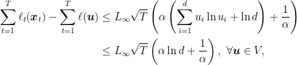
where we used the fact that using ${\psi_t=\alpha L_\infty \sqrt{t} \psi({\boldsymbol x})}$ and ${\psi_t=\alpha L_\infty \sqrt{t} (\psi({\boldsymbol x})-\min_{{\boldsymbol x}} \psi({\boldsymbol x}))}$ are equivalent. Choosing ${\alpha=\frac{1}{\sqrt{\ln d}}}$ . This regret guarantee is similar to the one we proved for OMD, but with an important difference: We don’t have to know in advance the number of rounds ${T}$ . In OMD a similar bound would be vacuous because it would depend on the ${\max_{{\boldsymbol u},{\boldsymbol x} \in V} B_\psi({\boldsymbol u};{\boldsymbol x})}$ that is infinite.

3. Composite Losses

Let’s now see a variant of the linearization of the losses: partial linearization of composite losses.

Suppose that the losses we receive are composed by two terms: one convex function changing over time and another part is fixed and known. These losses are called composite. For example, we might have ${\ell_t({\boldsymbol x})= \tilde{\ell}_t({\boldsymbol x})+\lambda \|{\boldsymbol x}\|_1}$ . Using the linearization, we might just take the subgradient of ${\ell_t}$ . However, in this particular case, we might lose the ability of the L1 norm to produce sparse solutions.

There is a better way to deal with these kind of losses: Move the constant part of the loss inside the regularization term. In this way, that part will not be linearized but used exactly in the argmin of the update. Assuming that the argmin is still easily computable, you can always expect better performance from this approach. In particular, in the case of adding an L1 norm to the losses, you will be predicting in each step with the solution of an L1 regularized optimization problem.

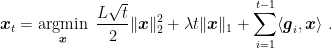
Practically speaking, in the example above, we will define ${\psi_t({\boldsymbol x}) = L \sqrt{t}(\psi({\boldsymbol x}) - \min_{{\boldsymbol y}} \ \psi({\boldsymbol y}))+ \lambda t \|{\boldsymbol x}\|_1}$ , where we assume ${\psi}$ to be 1-strongly convex and the losses ${\tilde{\ell}_t}$ be ${L}$ -Lipschitz. Note that we use at time ${t}$ a term ${\lambda t \|{\boldsymbol x}\|_1}$ because we anticipate the next term in the next round. Given that ${\psi_t({\boldsymbol x})+\sum_{i=1}^{t-1} \ell_t({\boldsymbol x})}$ is ${L \sqrt{t}}$ -strongly convex, using (1), we have

$\displaystyle \begin{aligned} \sum_{t=1}^T &\tilde{\ell}_t({\boldsymbol x}_t) - \sum_{t=1}^T \tilde{\ell}_t({\boldsymbol u}) \\ &\leq \sum_{t=1}^T \langle {\boldsymbol g}_t,{\boldsymbol x}_t\rangle - \sum_{t=1}^T \langle {\boldsymbol g}_t,{\boldsymbol u}\rangle \\ &\leq L \sqrt{T}\left(\psi({\boldsymbol u}) - \min_{{\boldsymbol x}} \ \psi(x)\right) + \lambda T \|{\boldsymbol u}\|_1 - \min_{{\boldsymbol x}} (\lambda \|{\boldsymbol x}\|_1 + \psi({\boldsymbol x})- \min_{{\boldsymbol y}} \ \psi({\boldsymbol y})) + \frac{1}{2}\sum_{t=1}^T \frac{\|{\boldsymbol g}_t\|^2_\star}{L \sqrt{t}} - \lambda \sum_{t=1}^{T-1} \|{\boldsymbol x}_{t+1}\|_1 \\ &\leq L \sqrt{T}\left(1+\psi({\boldsymbol u}) - \min_{{\boldsymbol x}} \ \psi(x) \right) + \lambda T \|{\boldsymbol u}\|_1 - \lambda \|{\boldsymbol x}_1\|_1 - \lambda \sum_{t=1}^{T-1} \|{\boldsymbol x}_{t+1}\|_1 \\ &= L \sqrt{T}\left(1+\psi({\boldsymbol u}) - \min_{{\boldsymbol x}} \ \psi(x) \right) + \lambda T \|{\boldsymbol u}\|_1 - \lambda \sum_{t=1}^{T} \|{\boldsymbol x}_{t}\|_1, \end{aligned}$

where ${{\boldsymbol g}_t \in \partial \tilde{\ell}_t({\boldsymbol x}_t)}$ . Reordering the terms, we have

$\displaystyle \sum_{t=1}^T \ell_t({\boldsymbol x}_t) - \sum_{t=1}^T \ell_t({\boldsymbol u}) = \sum_{t=1}^T (\lambda \|{\boldsymbol x}_t\|_1+\tilde{\ell}_t({\boldsymbol x}_t)) - \sum_{t=1}^T (\lambda \|{\boldsymbol u}\|_1+\tilde{\ell}_t({\boldsymbol u})) \leq L \sqrt{T}\left(\psi({\boldsymbol u}) - \min_{{\boldsymbol x}} \psi({\boldsymbol x})+ 1\right)~.$

Example 2 Let’s also take a look at the update rule in that case that ${\psi({\boldsymbol x})=\frac{1}{2}\|{\boldsymbol x}\|_2^2}$ and we get composite losses with the L1 norm. We have

$\displaystyle {\boldsymbol x}_{t} = \mathop{\mathrm{argmin}}_{{\boldsymbol x}} \ \frac{L\sqrt{t}}{2}\|{\boldsymbol x}\|_2^2 + \lambda t \|{\boldsymbol x}\|_1 + \sum_{i=1}^{t-1} \langle {\boldsymbol g}_i, {\boldsymbol x}\rangle~.$

We can solve this problem observing that the minimization decomposes over each coordinate of ${{\boldsymbol x}}$ . Denote by ${{\boldsymbol \theta}_t=\sum_{i=1}^{t-1} {\boldsymbol g}_i}$ . Hence, we know from first-order optimality condition that ${x_{t,i}}$ is the solution for the coordinate ${i}$ iff there exists ${v_i \in \partial |x_{t,i}|}$ such that

$\displaystyle L \sqrt{t} x_{t,i} + \lambda t v_i + \theta_{t,i} = 0$

Consider the 3 different cases:

${|\theta_{t,i}|\leq \lambda t}$ , then ${x_{t,i}=0}$ and ${v_i = - \tfrac{\theta}{\lambda t}}$ .

${\theta_{t,i}> \lambda t}$ , then ${x_{t,i}=-\frac{\theta_{t,i}-\lambda t}{L \sqrt{t}}}$ and ${v_i = - 1}$ .

${\theta_{t,i}< - \lambda t}$ , then ${x_{t,i}=-\frac{\theta_{t,i}+\lambda t}{L \sqrt{t}}}$ and ${v_i = 1}$ .

So, overall we have

$\displaystyle x_{t,i} = -\frac{\rm sign(\theta_{t,i})\max(|\theta_{t,i}|-\lambda t,0)}{L \sqrt{t}}~.$

Observe as this update will produce sparse solutions, while just taking the subgradient of the L1 norm would have never produced sparse predictions.

Remark 2 (Proximal operators) In the example above, we calculated something like

$\displaystyle \mathop{\mathrm{argmin}}_{{\boldsymbol x} \in {\mathbb R}^d} \ \|{\boldsymbol x}\|_1 - \langle{\boldsymbol v}, {\boldsymbol x}\rangle + \frac{1}{2}\|{\boldsymbol x}\|_2^2 =\mathop{\mathrm{argmin}}_{{\boldsymbol x} \in {\mathbb R}^d} \ \|{\boldsymbol x}\|_1 - \langle{\boldsymbol v}, {\boldsymbol x}\rangle + \frac{1}{2}\|{\boldsymbol x}\|_2^2 +\frac{1}{2}\|{\boldsymbol v}\|_2^2 =\mathop{\mathrm{argmin}}_{{\boldsymbol x} \in {\mathbb R}^d} \ \|{\boldsymbol x}\|_1 +\frac{1}{2}\|{\boldsymbol x}-{\boldsymbol v}\|_2^2~.$

This operation is known in the optimization literature as Proximal Operator of the L1 norm. In general, a proximal operator of a convex, proper, and closed function ${f:{\mathbb R}^d \rightarrow (-\infty,+\infty]}$ is defined as

$\displaystyle \text{Prox}_f({\boldsymbol v}) = \mathop{\mathrm{argmin}}_{{\boldsymbol x} \in {\mathbb R}^d} \ f({\boldsymbol x}) +\frac{1}{2}\|{\boldsymbol x}-{\boldsymbol v}\|_2^2~.$

Proximal operators are used in optimization in the same way as we used it: They allow to minimize the entire function rather a linear approximation of it. Also, proximal operators generalizes the concept of Euclidean projection. Indeed, ${\text{Prox}_{i_V}({\boldsymbol v})= \Pi_V({\boldsymbol v})}$ .

4. FTRL with Strongly Convex Functions

Let’s now go back to the FTRL regret bound and let’s see if you can strengthen it in the case that the regularizer is proximal, that is it satisfies that ${{\boldsymbol x}_t \in \mathop{\mathrm{argmin}}_{{\boldsymbol x}} \psi_{t+1}({\boldsymbol x})-\psi_t({\boldsymbol x})}$ .

Lemma 1 Denote by ${F_t({\boldsymbol x}) = \psi_{t}({\boldsymbol x}) + \sum_{i=1}^{t-1} \ell_i({\boldsymbol x})}$ . Assume that ${\mathop{\mathrm{argmin}}_{{\boldsymbol x} \in {\mathbb R}^d} \ F_{t}({\boldsymbol x})}$ is not empty and set ${{\boldsymbol x}_t \in \mathop{\mathrm{argmin}}_{{\boldsymbol x} \in {\mathbb R}^d} \ F_{t}({\boldsymbol x})}$ . Also, assume that ${F_t}$ is ${\lambda_t}$ -strongly convex w.r.t. ${\|\cdot\|}$ and ${\ell_t}$ convex, and the regularizer is such that ${{\boldsymbol x}_{t} \in \mathop{\mathrm{argmin}}_{{\boldsymbol x}} \psi_{t+1}({\boldsymbol x})-\psi_t({\boldsymbol x})}$ . Also, assume that ${\partial \ell_t({\boldsymbol x}_t)}$ is non-empty. Then, we have

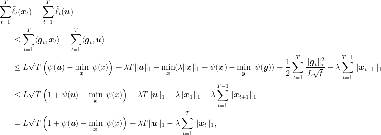
$\displaystyle F_t({\boldsymbol x}_t) - F_{t+1}({\boldsymbol x}_{t+1}) + \ell_t({\boldsymbol x}_t) \leq \frac{\|{\boldsymbol g}_t\|_*^2}{2\lambda_{t+1}} + \psi_t({\boldsymbol x}_t) - \psi_{t+1}({\boldsymbol x}_t), \ \forall {\boldsymbol g}_t \in \partial \ell_t({\boldsymbol x}_t)~.$

Proof: We have

$\displaystyle \begin{aligned} F_t&({\boldsymbol x}_t) - F_{t+1}({\boldsymbol x}_{t+1}) + \ell_t({\boldsymbol x}_t) \\ &= (F_t({\boldsymbol x}_t) + \ell_t({\boldsymbol x}_t) + \psi_{t+1}({\boldsymbol x}_t) - \psi_t({\boldsymbol x}_t)) - F_{t+1}({\boldsymbol x}_{t+1}) - \psi_{t+1}({\boldsymbol x}_t) + \psi_t({\boldsymbol x}_t)\\ &= F_{t+1}({\boldsymbol x}_t) - F_{t+1}({\boldsymbol x}_{t+1}) - \psi_{t+1}({\boldsymbol x}_t) + \psi_t({\boldsymbol x}_t)\\ &\leq \frac{\|{\boldsymbol g}'_t\|_*^2}{2\lambda_{t+1}} - \psi_{t+1}({\boldsymbol x}_t) + \psi_t({\boldsymbol x}_t), \end{aligned}$

where in the second inequality we used Corollary 1 from last lecture, the fact that ${{\boldsymbol x}_{t+1} = \mathop{\mathrm{argmin}}_{{\boldsymbol x}} \ F_{t+1}({\boldsymbol x})}$ , and ${{\boldsymbol g}'_t \in \partial F_{t+1}({\boldsymbol x}_t)}$ . Observing that from the proximal property, we have that ${{\boldsymbol x}_t = \mathop{\mathrm{argmin}}_{{\boldsymbol x}} F_t({\boldsymbol x}) + \psi_{t+1}({\boldsymbol x}) - \psi_t({\boldsymbol x})}$ , ${\boldsymbol{0} \in \partial (F_t({\boldsymbol x}_t)+ \psi_{t+1}({\boldsymbol x}_t) - \psi_t({\boldsymbol x}_t))}$ . Hence, using the theorem of the subdifferential of sum of functions, and remembering that ${F_{t+1}({\boldsymbol x})=F_{t}({\boldsymbol x}) + \ell_t({\boldsymbol x}) + \psi_{t+1}({\boldsymbol x}) - \psi_t({\boldsymbol x})}$ , we can choose ${{\boldsymbol g}'_t}$ such that we have ${{\boldsymbol g}'_t \in \partial \ell_t({\boldsymbol x}_t)}$ . $\Box$

Remark 3 Note that a constant regularizer is proximal because any point is the minimizer of the zero function. On the other hand, a constant regularizer makes the two Lemmas the same, unless the loss functions contribute to the total strong convexity.

We will now use the above lemma to prove a logarithmic regret bound for strongly convex losses.

Corollary 2 Let ${\ell_t}$ be ${\mu_t}$ strongly convex w.r.t. ${\|\cdot\|}$ , for ${t=1,\dots,T}$ . Set the sequence of regularizers to zero. Then, FTRL guarantees a regret of

$\displaystyle \sum_{t=1}^T \ell({\boldsymbol x}_t) - \sum_{t=1}^T \ell_t({\boldsymbol u}) \leq \frac{1}{2}\sum_{t=1}^T \frac{\|{\boldsymbol g}_t\|_\star^2}{\sum_{i=1}^t \mu_i}, \ \forall {\boldsymbol u} \in {\mathbb R}^d,\ \forall {\boldsymbol g}_t \in \partial \ell_t({\boldsymbol x}_t)~.$

The above regret guarantee is the same of OMD over strongly convex losses, but here we don’t need to know the strong convexity of the losses. In fact, we just need to output the minimizer over the past losses. However, as we noticed last time, this might be undesirable because now each update is an optimization problem.

Hence, we can again use the idea of replacing the losses with an easy surrogate. In the Lipschitz case, it made sense to use linear losses. However, here you can do better and use quadratic losses, because the losses are strongly convex. So, we can run FTRL on the quadratic losses ${\tilde{\ell}_t({\boldsymbol x})=\langle {\boldsymbol g}_t, {\boldsymbol x}\rangle + \frac{\mu_t}{2}\|{\boldsymbol x}-{\boldsymbol x}_t\|^2}$ , where ${{\boldsymbol g}_t \in \partial \ell_t({\boldsymbol x}_t)}$ . The algorithm would be the following one:

ftrl_algo_quad

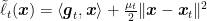
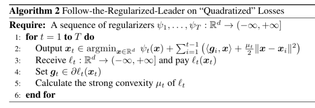
To see why this is a good idea, consider the case that the losses are strongly convex w.r.t. the L2 norm. The update now becomes:

$\displaystyle \label{eq:ftrl_upd_strongly} {\boldsymbol x}_t = \mathop{\mathrm{argmin}}_{{\boldsymbol x}} \sum_{i=1}^{t-1} \left(\langle {\boldsymbol g}_i, {\boldsymbol x}\rangle + \frac{\mu_i}{2}\|{\boldsymbol x}-{\boldsymbol x}_i\|_2^2\right) = \frac{\sum_{i=1}^{t-1} (\mu_i {\boldsymbol x}_i - {\boldsymbol g}_i)}{\sum_{i=1}^{t-1} \mu_i}~. \ \ \ \ \ (2)$

Moreover, we will get exactly the same regret bound as in Corollary 2, with the only difference that here the guarantee holds for a specific choice of the ${{\boldsymbol g}_t}$ rather than for any subgradient in ${\partial \ell_t({\boldsymbol x}_t)}$ .

Example 3 Going back to the example in the first lecture, where ${V=[0,1]}$ and ${\ell_t({\boldsymbol x})=(x-y_t)^2}$ are strongly convex, we now see immediately that FTRL without a regularizer, that is Follow the Leader, gives logarithmic regret. Note that in this case the losses were defined only over ${V}$ , so that the minimization is carried over ${V}$ .

5. History Bits

The first analysis of FTRL with composite losses is in (L. Xiao, 2010). The analysis presented here using the negative terms ${\psi_t({\boldsymbol x}_{t+1}) - \psi_{t+1}({\boldsymbol x}_{t+1})}$ to easily prove regret bounds for FTRL for composite losses is from (F. Orabona and K. Crammer and N. Cesa-Bianchi, 2015).

The first proof of FTRL for strongly convex losses was in (S. Shalev-Shwartz and Y. Singer, 2007) (even if they don’t call it FTRL).

There is an interesting bit about FTRL-Proximal (McMahan, H. B., 2011): FTRL-Proximal is an instantiation of FTRL that uses a particular proximal regularizer. It became very famous in internet companies when Google disclosed in a very influential paper that they were using FTRL-Proximal to train the classifier for click prediction (McMahan, H. B. and Holt, G. and Sculley, D. and Young, M. and Ebner, D. and Grady, J. and Nie, L. and Phillips, T. and Davydov, E. and Golovin, D. and Chikkerur, S. and Liu, D. and Wattenberg, M. and Hrafnkelsson, A. M. and Boulos, T. and Kubica, J., 2013). This generated even more confusion because many people started conflating the term FTRL-Proximal (a specific algorithm) with FTRL (an entire family of algorithms). Unfortunately, this confusion is still going on in these days.

6. Exercises

Exercise 1 Prove that the update in (2) is equivalent to the one of OSD with ${{\boldsymbol x}_1=0}$ and learning rate ${\eta_t=\frac{1}{\sum_{i=1}^t \mu_t}}$ .

4 Comments

Pingback: Follow-The-Regularized-Leader III: More Logarithmic Bounds – Parameter-free Learning and Optimization Algorithms
mihahauke says:

September 30, 2020 at 7:06 AM

What do you mean exactly by “proximal regularizer”? I imagined that one that includes euclidean distance from x_t but even if it were true I don’t know how to derive x_t \in argmin_x \psi_{t+1}(x) – \psi_t(x).

LikeLike

1. bremen79 says:
  
  September 30, 2020 at 12:15 PM
  
  It is just a technical condition introduced by Brendan McMahan. There are not many algorithms that actually have a proximal regularizers, but constant regularizer is proximal. So, I used it because it allows me to deal with a bunch of different cases with one Lemma. In the note on Online Newton Step, for example, I used this characterization again.
  
  LikeLike
  
Pingback: Implicit, Passive-Aggressive, and aProx updates – Parameter-free Learning and Optimization Algorithms
anonima says:

May 25, 2023 at 10:54 AM

When proving that FTRL with linerized losses is equivalent to OMD, at the very first steps there is “Assume x_{t+1} is in the int dom psi , then ngt-\/psi(x_t+1)-\/psi(x_t) = 0. Is there any resource to study why this holds?

LikeLike

bremen79 says:

May 25, 2023 at 11:04 AM

There, I am assuming V=dom psi. So, if the update of OMD is in int dom psi it means that the constraint did not play any role. In other words, you would obtain the same update removing completely the feasible set. This implies that x_{t+1} is the unconstrained minimum of the OMD update rule, hence the gradient of the OMD update rule must be 0 in x_{t+1}, that is exactly the equality I wrote.

LikeLike