Multi-Armed Bandit I

This post is part of the lecture notes of my class “Introduction to Online Learning” at Boston University, Fall 2019. I will publish two lectures per week.

You can find the lectures I published till now here.

Today, we will present the problem of multi-armed bandit in the adversarial setting and show how to obtain sublinear regret.

1. Multi-Armed Bandit

This setting is similar to the Learning with Expert Advice (LEA) setting: In each round, we select one expert ${A_t}$ and, differently from the full-information setting, we only observe the loss of that expert ${g_{t,i}}$ . The aim is still to compete with the cumulative loss of the best expert in hindsight.

As in the learning with expert case, we need randomization in order to have a sublinear regret. Indeed, this is just a harder problem than LEA. However, we will assume that the adversary is oblivious, that is, he decides the losses of all the rounds before the game starts, but with the knowledge of the online algorithm. This makes the losses deterministic quantities and it avoids the inadequacy in our definition of regret when the adversary is adaptive (see (Arora, R. and Dekel, O. and Tewari, A., 2012)).

This kind of problems where we don’t receive the full-information, i.e., we don’t observe the loss vector, are called bandit problems. The name comes from the problem of a gambler who plays a pool of slot machines, that can be called “one-armed bandits”. On each round, the gambler places his bet on a slot machine and his goal is to win almost as much money as if he had known in advance which slot machine would return the maximal total reward.

In this problem, we clearly have an exploration-exploitation trade-off. In fact, on one hand we would like to play at the slot machine which, based on previous rounds, we believe will give us the biggest win. On the other hand, we have to explore the slot machines to find the best ones. On each round, we have to solve this trade-off.

Given that we don’t observe completely observe the loss, we cannot use our two frameworks: Online Mirror Descent (OMD) and Follow-The-Regularized-Leader (FTRL) both needs the loss functions or at least lower bounds to them.

One way to solve this issue is to construct stochastic estimates of the unknown losses. This is a natural choice given that we already know that the prediction strategy has to be a randomized one. So, in each round ${t}$ we construct a probability distribution over the arms ${{\boldsymbol x}_t}$ and we sample one action ${A_t}$ according to this probability distribution. Then, we only observe the coordinate ${A_t}$ of the loss vector ${{\boldsymbol g}_t \in {\mathbb R}^d}$ . One possibility to have a stochastic estimate of the losses is to use an importance-weighted estimator: Construct the estimator ${\tilde{{\boldsymbol g}}_t}$ of the unknown vector ${{\boldsymbol g}_t}$ in the following way:

$\displaystyle \tilde{{\boldsymbol g}}_t=\begin{cases} \frac{g_{t,i}}{x_{t,i}}, & i=A_t\\ 0, & \text{ otherwise}\end{cases}~.$

Note that this estimator has all the coordinates equal to 0, except the coordinate corresponding the arm that was pulled.

This estimator is unbiased, that is ${\mathop{\mathbb E}_{A_t}[\tilde{{\boldsymbol g}}_t]={\boldsymbol g}_t}$ . To see why, note that ${\tilde{g}_{t,i} = \boldsymbol{1}[A_t=i]\frac{g_{t,i}}{x_{t,i}}}$ and ${\mathop{\mathbb E}_{A_t}[\boldsymbol{1}[A_t=i]]=x_{t,i}}$ . Hence, for ${i=1, \dots, d}$ , we have

$\displaystyle \mathop{\mathbb E}_{A_t}[\tilde{g}_{t,i}] = \mathop{\mathbb E}_{A_t}\left[\boldsymbol{1}[A_t=i]\frac{g_{t,i}}{x_{t,i}}\right] = \frac{g_{t,i}}{x_{t,i}} \mathop{\mathbb E}_{A_t}[\boldsymbol{1}[A_t=i]] = g_{t,i}~.$

Let’s also calculate the (uncentered) variance of the coordinates of this estimator. We have

$\displaystyle \mathop{\mathbb E}_{A_t}[\tilde{g}_{t,i}^2] = \mathop{\mathbb E}_{A_t}\left[\boldsymbol{1}[A_t=i]\frac{g^2_{t,i}}{x^2_{t,i}}\right] = \frac{g_{t,i}^2}{x_{t,i}}~.$

We can now think of using OMD with an entropic regularizer and the estimated losses. Hence, assume ${\|{\boldsymbol g}_t\|_\infty\leq L_\infty}$ and set ${\psi:{\mathbb R}^d_+ \rightarrow {\mathbb R}}$ defined as ${\psi({\boldsymbol x})=\sum_{i=1}^d x_i \ln x_i}$ , that is the unnormalized negative entropy. Also, set ${{\boldsymbol x}_1=[1/d, \dots, 1/d]}$ . Using the OMD analysis, we have

$\displaystyle \sum_{t=1}^T \langle \tilde{{\boldsymbol g}}_t,{\boldsymbol x}_t\rangle - \sum_{t=1}^T \langle \tilde{{\boldsymbol g}}_t,{\boldsymbol u}\rangle \leq \frac{\ln d}{\eta} + \frac{\eta}{2}\sum_{t=1}^T \|\tilde{{\boldsymbol g}}_t\|_\infty^2~.$

We can now take the expectation at both sides and get

$\displaystyle \begin{aligned} \mathop{\mathbb E}\left[\sum_{t=1}^T g_{t,A_t}\right] - \sum_{t=1}^T \langle {\boldsymbol g}_t,{\boldsymbol u}\rangle &=\mathop{\mathbb E}\left[\sum_{t=1}^T \langle {\boldsymbol g}_t,{\boldsymbol x}_t\rangle\right] - \sum_{t=1}^T \langle {\boldsymbol g}_t,{\boldsymbol u}\rangle & (1) \\ &=\mathop{\mathbb E}\left[\sum_{t=1}^T \langle \tilde{{\boldsymbol g}}_t,{\boldsymbol x}_t\rangle - \sum_{t=1}^T \langle \tilde{{\boldsymbol g}}_t,{\boldsymbol u}\rangle\right] \\ &\leq \frac{\ln d}{\eta} + \frac{\eta}{2}\sum_{t=1}^T \mathop{\mathbb E}[\|\tilde{{\boldsymbol g}}_t\|_\infty^2] \\ &\leq \frac{\ln d}{\eta} + \frac{\eta}{2}\sum_{t=1}^T \sum_{i=1}^d \frac{g_{t,i}^2}{x_{t,i}}~. & (2) \\\end{aligned}$

We are now in troubles, because the terms in the sum scale as ${\max_{i=1,\dots,d} \ \frac{1}{x_{t,i}}}$ . So, we need a way to control the smallest probability over the arms.

One way to do it, is to take a convex combination of ${{\boldsymbol x}_t}$ and a uniform probability. That is, we can predict with ${\tilde{{\boldsymbol x}}_t=(1-\alpha) {\boldsymbol x}_t + \alpha [1/d, \dots, 1/d]}$ , where ${\alpha}$ will be chosen in the following. So, ${\alpha}$ can be seen as the minimum amount of exploration we require to the algorithm. Its value will be chosen by the regret analysis to optimally trade-off exploration vs exploitation. The resulting algorithm is in Algorithm 1.

eg_bandit

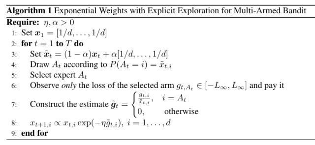
The same probability distribution is used in the estimator:

$\displaystyle \label{eq:tilde_bg_t} \tilde{{\boldsymbol g}}_t=\begin{cases} \frac{g_{t,i}}{\tilde{x_{t,i}}}, & i=A_t\\ 0, & \text{ otherwise}\end{cases}~. \ \ \ \ \ (3)$

We can have that ${\frac{1}{\tilde{x}_{t,i}}\leq \frac{d}{\alpha}}$ . However, we pay a price in the bias introduced:

$\displaystyle \sum_{t=1}^T \langle \tilde{{\boldsymbol g}}_t, \tilde{{\boldsymbol x}}_t-{\boldsymbol u}\rangle = \sum_{t=1}^T \langle \tilde{{\boldsymbol g}}_t, (1-\alpha){\boldsymbol x}_t - {\boldsymbol u}\rangle + \frac{\alpha}{d} \sum_{t=1}^T \sum_{i=1}^d \tilde{g}_{t,i}~.$

Observing that ${\mathop{\mathbb E}[\sum_{i=1}^d \tilde{g}_{t,i}]=\sum_{i=1}^d g_{t,i}\leq d L_\infty}$ , we have

$\displaystyle \mathop{\mathbb E}\left[\sum_{t=1}^T \langle \tilde{{\boldsymbol g}}_t, \tilde{{\boldsymbol x}}_t-{\boldsymbol u}\rangle \right] \leq \mathop{\mathbb E}\left[\sum_{t=1}^T \langle \tilde{{\boldsymbol g}}_t, (1-\alpha){\boldsymbol x}_t-{\boldsymbol u}\rangle \right] + \alpha L_\infty T \leq \mathop{\mathbb E}[\text{Regret}_T({\boldsymbol u})] + \alpha L_\infty T~.$

Putting together the last inequality and the upper bound to the expected regret in (2), we have

$\displaystyle \mathop{\mathbb E}\left[\sum_{t=1}^T g_{t,A_t}\right] - \sum_{t=1}^T \langle {\boldsymbol g}_t,{\boldsymbol u}\rangle \leq \frac{\ln d}{\eta} + \frac{\eta d^2 L_\infty^2 T}{2 \alpha} + \alpha L_\infty T~.$

Setting ${\alpha \propto \sqrt{d^2 L_\infty \eta}}$ and ${\eta \propto \left(\frac{\ln d}{d L_\infty^{3/2} T}\right)^{2/3}}$ , we obtain a regret of ${O(L_\infty (d T)^{2/3} \ln^{1/3} d )}$ .

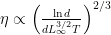
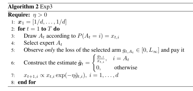
This is way worse than the ${O(\sqrt{T \ln d})}$ of the full-information case. However, while it is expected that the bandit case must be more difficult than the full information one, it turns out that this is not the optimal strategy.

2. Exponential-weight algorithm for Exploration and Exploitation: Exp3

It turns out that the algorithm above actually works, even without the mixing with the uniform distribution! We were just too loose in our regret guarantee. So, we will analyse the following algorithm, that is called Exponential-weight algorithm for Exploration and Exploitation (Exp3), that is nothing else than OMD with entropic regularizer and stochastic estimates of the losses. Note that now we will assume that ${g_{t,i} \in [0, L_\infty]}$ .

exp3

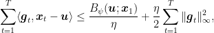
Let’s take another look to the regret guarantee we have. From the OMD analysis, we have the following one-step inequality that holds for any ${{\boldsymbol g}_t}$

$\displaystyle \langle \eta {\boldsymbol g}_t, {\boldsymbol x}_t - {\boldsymbol u}\rangle \leq B_\psi({\boldsymbol u};{\boldsymbol x}_t) - B_\psi({\boldsymbol u};{\boldsymbol x}_{t+1}) - B_\psi({\boldsymbol x}_{t+1};{\boldsymbol x}_t) + \langle \eta {\boldsymbol g}_t, {\boldsymbol x}_t - {\boldsymbol x}_{t+1} \rangle~.$

Let’s now focus on the term ${-B_\psi({\boldsymbol x}_{t+1};{\boldsymbol x}_t)+\langle \eta {\boldsymbol g}_t, {\boldsymbol x}_t - {\boldsymbol x}_{t+1}\rangle}$ . We said that for a twice differentiable function ${f}$ , there exists ${\alpha \in [0,1]}$ such that ${B_f({\boldsymbol x};{\boldsymbol y})=\frac12 ({\boldsymbol x}-{\boldsymbol y})^\top \nabla^2 f({\boldsymbol z}) ({\boldsymbol x}-{\boldsymbol y})}$ , where ${{\boldsymbol z}=\alpha {\boldsymbol x}+(1-\alpha) {\boldsymbol y}}$ . Hence, there exists ${\alpha_t\in[0,1]}$ such that ${{\boldsymbol z}_t=\alpha_t {\boldsymbol x}_t+(1-\alpha_t) {\boldsymbol x}_{t+1}}$ and

$\displaystyle B_\psi({\boldsymbol x}_{t+1};{\boldsymbol x}_t) =\frac12 ({\boldsymbol x}_t-{\boldsymbol x}_{t+1})^\top \nabla^2 \psi({\boldsymbol z}_t) ({\boldsymbol x}_t-{\boldsymbol x}_{t+1}) =\frac{1}{2}\|{\boldsymbol x}_t-{\boldsymbol x}_{t+1}\|^2_{\nabla^2 \psi({\boldsymbol z}_t)}~.$

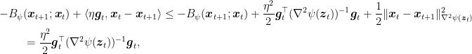
So, assuming the Hessian in ${{\boldsymbol z}_t}$ to be positive definite, we can bound the last two terms in the one-step inequality of OMD as

$\displaystyle \begin{aligned} -B_\psi&({\boldsymbol x}_{t+1};{\boldsymbol x}_t)+\langle \eta {\boldsymbol g}_t, {\boldsymbol x}_t - {\boldsymbol x}_{t+1}\rangle \leq -B_\psi({\boldsymbol x}_{t+1};{\boldsymbol x}_t) + \frac{\eta^2}{2} {\boldsymbol g}_t^\top (\nabla^2 \psi({\boldsymbol z}_t))^{-1} {\boldsymbol g}_t + \frac{1}{2}\|{\boldsymbol x}_t-{\boldsymbol x}_{t+1}\|^2_{\nabla^2 \psi({\boldsymbol z}_t)} \\ &= \frac{\eta^2}{2} {\boldsymbol g}_t^\top (\nabla^2 \psi({\boldsymbol z}_t))^{-1} {\boldsymbol g}_t, \end{aligned}$

where we used Fenchel-Young inequality with the function ${f({\boldsymbol x})=\frac12 \|{\boldsymbol x}\|^2_{\nabla^2 \psi({\boldsymbol x}_t)}}$ and ${{\boldsymbol z}_t=\alpha_t {\boldsymbol x}_t+(1-\alpha_t) {\boldsymbol x}_{t+1}}$ and ${\alpha_t\in[0,1]}$ .

simplex3 — Figure 1. Contour plots of the KL divergence in 3-dimensions when ${{\boldsymbol x}_t=[1/3,1/3,1/3]}$ (left) and when ${{\boldsymbol x}_t=[0.1,0.45,0.45]}$ (right).

Figure 1. Contour plots of the KL divergence in 3-dimensions when ${{\boldsymbol x}_t=[1/3,1/3,1/3]}$ (left) and when ${{\boldsymbol x}_t=[0.1,0.45,0.45]}$ (right).

When we use the strong convexity, we are upper bounding the terms in the sum with the inverse of the smallest eigenvalue of the Hessian of the regularizer. However, we can do better if we consider the actual Hessian. In fact, in the coordinates where ${{\boldsymbol x}_{t}}$ is small, we have a smaller growth of the divergence. This can be seen also graphically in Figure 1. Indeed, for the entropic regularizer, we have that the Hessian is a diagonal matrix:

$\displaystyle (\nabla^2 \psi({\boldsymbol z}))_{ii} = \frac{1}{z_i} \ i=1, \dots, d~.$

This expression of the Hessian a regret of

$\displaystyle \sum_{t=1}^T \langle {\boldsymbol g}_t, {\boldsymbol x}_t - {\boldsymbol u}\rangle \leq \frac{B_\psi({\boldsymbol u}; {\boldsymbol x}_1)}{\eta} + \frac{\eta}{2} \sum_{t=1}^T \sum_{i=1}^d z_{t,i} g_{t,i}^2,$

where ${{\boldsymbol z}_t=\alpha_t {\boldsymbol x}_t+(1-\alpha_t) {\boldsymbol x}_{t+1}}$ and ${\alpha_t\in[0,1]}$ . Note that for any ${\alpha_t \in [0,1]}$ ${{\boldsymbol z}_t}$ is in the simplex, so this upper bound is always better than

that we derived just using the strong convexity of the entropic regularizer.

However, we don’t know the exact value of ${{\boldsymbol z}_t}$ , but only that it is on the line segment between ${{\boldsymbol x}_t}$ and ${{\boldsymbol x}_{t+1}}$ . Yet, if you could say that ${z_{t,i}=O(x_{t,i})}$ , in the bandit case we would obtain an expected regret guarantee of ${O(\sqrt{d T \ln d})}$ , greatly improving the bound we proved above!

In the next lecture, we will see an alternative way to analyze OMD that will give us exactly this kind of guarantee for Exp3 and will use give us the optimal regret guarantee using the Tsallis entropy in few lines of proof.

3. History Bits

The algorithm in Algorithm 1 is from (Cesa-Bianchi, N. and Lugosi, G. , 2006, Theorem 6.9). The Exp3 algorithm was proposed in (Auer, P. and Cesa-Bianchi, N. and Freund, Y. and Schapire, R. E., 2002).