Parameter-free Online Learning III: from Coins to Experts

This post is part of the lecture notes of my class “Introduction to Online Learning” at Boston University, Fall 2019. I will publish two lectures per week.

You can find the lectures I published till now here.

In the last lecture, we have shown a very simple and parameter-free algorithm for Online Convex Optimization (OCO) in ${d}$ -dimensions, based on a reduction to a coin-betting problem. Now, we will see how to reduce Learning with Expert Advice (LEA) to betting on ${d}$ coins, obtaining again parameter-free and optimal algorithms.

1. Reduction to Learning with Experts

First, remember that the regret we got from Online Mirror Descent (OMD), and similarly for Follow-The-Regularized-Leader (FTRL), is

$\displaystyle \text{Regret}_T({\boldsymbol u}) \leq O\left(\frac{KL({\boldsymbol u};{\boldsymbol \pi})}{\eta} + \eta T \right),$

where ${{\boldsymbol \pi}}$ is the prior distribution on the experts and ${KL(\cdot; \cdot)}$ is the KL-divergence. As we reasoned in the OCO case, in order to set the learning rate we should know the value of ${KL({\boldsymbol u};{\boldsymbol \pi})}$ . If we could set ${\eta}$ to ${\sqrt{\frac{KL({\boldsymbol u};{\boldsymbol \pi})}{T}}}$ , we would obtain a regret of ${\sqrt{T\, KL({\boldsymbol u}; {\boldsymbol \pi})}}$ . However, given the adversarial nature of the game, this is impossible. So, as we did in the OCO case, we will show that even this problem can be reduced to betting on a coin, obtaining optimal guarantees with a parameter-free algorithm.

First, let’s introduce some notation. Let ${d \ge 2}$ be the number of experts and ${\Delta^d}$ be the ${d}$ -dimensional probability simplex. Let ${{\boldsymbol \pi} = [\pi_1, \pi_2, \dots, \pi_d] \in \Delta^d}$ be any prior distribution. Let ${\mathcal{A}}$ be a coin-betting algorithm. We will instantiate ${d}$ copies of ${\mathcal{A}}$ .

Consider any round ${t}$ . Let ${x_{t,i} \in {\mathbb R}}$ be the bet of the ${i}$ -th copy of ${\mathcal{A}}$ . The LEA algorithm computes ${\widehat {\boldsymbol p}_t = [\widehat p_{t,1}, \widehat p_{t,2}, \dots, \widehat p_{t,d}] \in {\mathbb R}_{+}^d}$ as

$\displaystyle \label{eq:phat} \widehat p_{t,i} = \pi_i \cdot \max(x_{t,i},0)~. \ \ \ \ \ (1)$

Then, the LEA algorithm predicts ${{\boldsymbol p}_t = [p_{t,1}, p_{t,2}, \dots, p_{t,d}] \in \Delta^d}$ as

$\displaystyle \label{eq:preds_experts} {\boldsymbol p}_t = \begin{cases} \tfrac{\widehat {\boldsymbol p}_t}{\|\widehat {\boldsymbol p}_t\|_1}, & \text{ if } \widehat {\boldsymbol p}_t\neq \boldsymbol{0}, \\ {\boldsymbol \pi}, & \text{ otherwise}~. \end{cases} \ \ \ \ \ (2)$

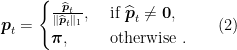
Then, the algorithm receives the reward vector ${{\boldsymbol g}_t = [g_{t,1}, g_{t,2}, \dots, g_{t,d}] \in [0,1]^d}$ . Finally, it feeds the reward to each copy of ${\mathcal{A}}$ . The reward for the ${i}$ -th copy of ${\mathcal{A}}$ is ${c_{t,i} \in [-1,1]}$ defined as

$\displaystyle \label{eq:gradients_experts_reduction} c_{t,i} = \begin{cases} \langle {\boldsymbol g}_t, {\boldsymbol p}_t \rangle - g_{t,i} & \text{if } x_{t,i} > 0, \\ \max\left(\langle {\boldsymbol g}_t, {\boldsymbol p}_t \rangle - g_{t,i} , 0\right) & \text{if } x_{t,i} \le 0~. \end{cases} \ \ \ \ \ (3)$

The construction above defines a LEA algorithm defined by the predictions ${{\boldsymbol p}_t}$ , based on the algorithm ${\mathcal{A}}$ . We can prove the following regret bound for it.

Theorem 1 (Regret Bound for Experts) Let ${\mathcal{A}}$ be a coin-betting algorithm that guarantees a wealth after ${t}$ rounds with initial money equal to 1 of 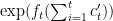${\exp(f_t(\sum_{i=1}^t c'_t))}$ for any sequence of continuous coin outcomes ${c'_1, \dots, c't \in [-1,1]}$ . Then, the regret of the LEA algorithm with prior ${\pi \in \Delta^d}$ that predicts at each round with ${{\boldsymbol p}_t}$ in (2) satisfies

$\displaystyle \forall T \ge 0, \quad \forall {\boldsymbol u} \in \Delta^d, \qquad \qquad \text{Regret}_T({\boldsymbol u}) = \sum_{t=1}^T \langle {\boldsymbol g}_t, {\boldsymbol p}_t -{\boldsymbol u}\rangle \le h\left( KL({\boldsymbol u};{\boldsymbol \pi}) \right),$

for any ${h:{\mathbb R}\rightarrow{\mathbb R}}$ concave and non-decreasing such that ${x\leq h(f_T(x))}$ .

Proof: We first prove that ${\sum_{i=1}^d \pi_i c_{t,i} x_{t,i} \le 0}$ . Indeed,

$\displaystyle \begin{aligned} \sum_{i=1}^d \pi_i c_{t,i} x_{t,i} & = \sum_{i \, : \, \pi_i x_{t,i} > 0} \pi_i \max(x_{t,i},0) (\langle {\boldsymbol g}_t, {\boldsymbol p}_t \rangle-g_{t,i}) \ + \ \sum_{i \, : \, \pi_i x_{t,i} \le 0} \pi_i x_{t,i} \max(\langle {\boldsymbol g}_t, {\boldsymbol p}_t \rangle - g_{t,i} ,0) \\ & = \|\widehat {\boldsymbol p}_t\|_1 \sum_{i=1}^d p_{t,i} (\langle {\boldsymbol g}_t, {\boldsymbol p}_t \rangle - {\boldsymbol g}_{t,i} ) \ + \ \sum_{i \, : \, \pi_i x_{t,i} \le 0} \pi_i x_{t,i} \max(\langle {\boldsymbol g}_t, {\boldsymbol p}_t\rangle - g_{t,i} ,0) \\ & = 0 \ + \ \sum_{i \, : \, \pi_i x_{t,i} \le 0} \pi_i x_{t,i} \max(\langle {\boldsymbol g}_t, {\boldsymbol p}_t\rangle - g_{t,i} ,0) \ \le 0 \; . \end{aligned}$

The first equality follows from definition of ${c_{t,i}}$ . To see the second equality, consider two cases: If ${\pi_i x_{t,i} \le 0}$ for all ${i}$ then ${\|\widehat p_t\|_1 = 0}$ and therefore both 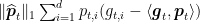${\|\widehat {\boldsymbol p}_t\|_1 \sum_{i=1}^d p_{t,i} (g_{t,i} - \langle {\boldsymbol g}_t, {\boldsymbol p}_t \rangle)}$ and ${\sum_{i \, : \, \pi_i x_{t,i} > 0} \pi_i \max(w_{t,i},0) (g_{t,i} - \langle {\boldsymbol g}_t, {\boldsymbol p}_t \rangle)}$ are trivially zero. If ${\|\widehat {\boldsymbol p}_t\|_1 > 0}$ then ${\pi_i \max(x_{t,i},0) = \widehat p_{t,i} = \|\widehat {\boldsymbol p}_t\|_1 p_{t,i}}$ for all ${i}$ .

From the assumption on ${\mathcal{A}}$ , we have for any sequence ${\{c'_t\}_{t=1}^T}$ such that ${c'_t \in [-1,1]}$ that

$\displaystyle \label{equation:experts-one-dimensional-assumption} \text{Wealth}_T = 1 + \sum_{t=1}^T c'_t x_t \ge \exp\left(f_T\left(\sum_{t=1}^T c'_t\right)\right)~. \ \ \ \ \ (4)$

So, inequality ${\sum_{i=1}^d \pi_i c_{t,i} x_{t,i} \le 0}$ and (4) imply

$\displaystyle \label{equation:bounded-potential} \sum_{i=1}^d \pi_i \exp\left(f_T \left(\sum_{t=1}^T c_{t,i} \right)\right) \le 1 + \sum_{i=1}^d \pi_i \sum_{t=1}^T c_{t,i} x_{t,i} \le 1~ . \ \ \ \ \ (5)$

Now, for any competitor ${{\boldsymbol u} \in \Delta^d}$ ,

$\displaystyle \begin{aligned} \text{Regret}_T({\boldsymbol u}) &= \sum_{t=1}^T \langle {\boldsymbol g}_t, {\boldsymbol p}_t - {\boldsymbol u} \rangle \\ &= \sum_{t=1}^T \sum_{i=1}^d u_i \left(\langle {\boldsymbol g}_t, {\boldsymbol p}_t \rangle - g_{t,i} \right) \\ & \le \sum_{t=1}^T \sum_{i=1}^N u_i c_{t,i} \qquad \text{(by definition of } c_{t,i} \text{)} \\ & \leq \sum_{i=1}^N u_i h\left(f_T\left( \sum_{t=1}^T c_{t,i}\right) \right) \qquad \text{(definition of the } h(x) \text{)} \\ & \le h\left[\sum_{i=1}^N u_i f_T\left( \sum_{t=1}^T c_{t,i}\right) \right] \qquad \text{(by concavity of } h \text{ and Jensen inequality)} \\ & \le h\left[KL({\boldsymbol u};{\boldsymbol \pi})+\ln \left(\sum_{i=1}^N \pi_i \exp\left(f_T\left(\sum_{t=1}^T c_{t,i}\right)\right) \right)\right] \qquad \text{(Fenchel-Young inequality)} \\ & \le h(KL({\boldsymbol u};{\boldsymbol \pi})) \qquad \text{(by (5))}~. \end{aligned}$

$\Box$

Now, we could think to use the Krichevsky–Trofimov (KT) bettor with this theorem. However, we would obtain a sub-optimal regret guarantee. In fact, remembering the lower bound on the wealth of KT and setting ${h(x)=\sqrt{4T(x+\frac12 \ln T + K )}}$ where ${K}$ is a universal constant, we have

$\displaystyle \text{Regret}_T({\boldsymbol u}) \leq O(\sqrt{T(KL({\boldsymbol u};{\boldsymbol \pi})+\ln T)})~.$

We might think that the ${\ln T}$ is the price we have to pay to adapt to the unknown competitor ${{\boldsymbol u}}$ . However, it turns out it can be removed. In the next section, we see how to change the KT strategy to obtain the optimal guarantee.

2. A Betting Strategy that Looses at Most a Constant Fraction of Money

In the reduction before, if we use the KT betting strategy we would have a ${\ln T}$ term under the square root. It turns out that we can avoid that term if we know the number of rounds beforehand. Then, in case ${T}$ is unknown we can just use a doubling trick, paying only a constant multiplicative factor in the regret.

The logarithmic term in the regret comes from the fact that the lower bound on the wealth is

$\displaystyle O\left(\frac{1}{\sqrt{T}}\exp\left(\frac{(\sum_{t=1}^T c_t)^2}{4T}\right)\right)~.$

Note that in the case in which the number of heads in the sequence is equal to the number of heads, so that ${\sum_{t=1}^T c_t=0}$ , the guaranteed wealth becomes proportional to ${\frac{1}{\sqrt{T}}}$ . So, for ${T}$ that goes to infinity the bettor will lose all of its money.

Instead, we need a more conservative strategy that guarantees

$\displaystyle O\left(\alpha\exp\left(\frac{(\sum_{t=1}^T c_t)^2}{4 T}\right)\right),$

for ${\alpha}$ small enough and independent of ${T}$ . In this case, the betting strategy has to pace its betting, possibly with the knowledge of the duration of the game, so that even in the case that the number of heads is equal to the number of tails it will only lose a fraction of its money. At the same time, it will still gain an exponential amount of money when the coin outcomes are biased towards one side.

We will prove that this is possible, designing a new betting strategy.

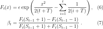
Denote by ${S_{t}=\sum_{i=1}^{t} c_i}$ for ${t=1, \dots, T}$ and define

$\displaystyle \begin{aligned} F_t(x)&=\epsilon \exp\left(\frac{x^2}{2(t+T)} - \sum_{i=1}^{t} \frac{1}{2(i+T)}\right), & (6) \\ \beta_t&=\frac{F_{t}(S_{t-1}+1)-F_{t}(S_{t-1}-1)}{F_{t}(S_{t-1}+1)+F_{t}(S_{t-1}-1)}~.& (7) \\\end{aligned}$

Note that if

$\displaystyle \label{eq:property_betting_potentials} (1+\beta_t c_t) F_{t-1}\left(\sum_{i=1}^{t-1} c_i\right) \geq F_{t}\left(\sum_{i=1}^{t} c_i\right) \ \ \ \ \ (8)$

then, by induction, ${\text{Wealth}_T \geq F_{T}\left(\sum_{t=1}^{T} c_t\right)}$ . In fact, we have

$\displaystyle \text{Wealth}_{t} = (1+\beta_t c_t) \text{Wealth}_{t-1} \geq (1+\beta_t c_t) F_{t-1} \left(\sum_{i=1}^{t-1} c_i\right) \geq F_{t}\left(\sum_{i=1}^{t} c_i\right)~.$

Hence, we have to prove that (8) is true in order to guarantee a minimum wealth of our betting strategy.

First, given that 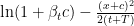${\ln(1+\beta_t c) - \frac{(x+c)^2}{2(t+T)}}$ is a concave function of ${c}$ , we have

$\displaystyle \min_{ c \in [-1,1]} \ \ln(1+\beta_t c) - \frac{(x+c)^2}{2(t+T)} = \min\left(\ln(1+\beta_t) - \frac{(x+1)^2}{2(t+T)}, \ln(1-\beta_t) - \frac{(x-1)^2}{2(t+T)}\right)~.$

Also, our choice of ${\beta_t}$ makes the two quantities above equal with ${x=S_{t-1}}$ , that is

$\displaystyle \ln(1+\beta_t) - \ln F_t (S_{t-1} + 1) = \ln(1-\beta_t) - \ln F_t (S_{t-1} - 1)$

For other choices of ${\beta_t}$ , the two alternatives would be different and the minimum one could always be the one picked by the adversary. Instead, making the two choices worst outcomes equivalent, we minimize the damage of the adversarial choice of the outcomes of the coin. So, we have that

$\displaystyle \begin{aligned} \ln (1+\beta_t c_t) - \ln F_t(S_t) &= \ln (1+\beta_t c_t) + F_t(S_{t-1}+c_t) \\ &\geq \min_{ c \in [-1,1]} \ \ln (1+\beta_t c) + \ln F_t(S_{t-1}+c) \\ &= -\ln \frac{F_{t}(S_{t-1}+1)+F_{t}(S_{t-1}-1)}{2} \\ &=- \ln \left[\exp\left(\frac{S_{t-1}^2+1}{2(t+T)} - \sum_{i=1}^t \frac{1}{2(i+T)}\right) \frac{1}{2}\left(\exp\left(\frac{S_{t-1}}{t+T}\right) + \exp\left(\frac{-S_{t-1}}{t+T}\right) \right) \right] \\ &= -\frac{S_{t-1}^2+1}{2(t+T)} - \ln \cosh\frac{S_{t-1}}{t+T} + \sum_{i=1}^t \frac{1}{2(i+T)} \\ &\geq -\frac{S_{t-1}^2}{2(t+T)} - \frac{S_{t-1}^2}{2(t+T)^2} + \sum_{i=1}^{t-1} \frac{1}{2(i+T)} \\ &\geq -\frac{S_{t-1}^2}{2(t+T)} - \frac{S_{t-1}^2}{2(t+T)(t-1+T)} + \sum_{i=1}^{t-1} \frac{1}{2(i+T)} \\ &= -\frac{S_{t-1}^2}{2(t-1+T)}+ \sum_{i=1}^{t-1} \frac{1}{2(i+T)} \\ &= -\ln F_{t-1}(S_{t-1}), \end{aligned}$

where in the second equality we used the definition of ${\beta_t}$ and in the second inequality we used the fact that ${\ln \cosh(x)\leq \frac{x^2}{2}, \forall x}$ .

Hence, given that (8) is true, this strategy guarantees

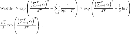
$\displaystyle \text{Wealth}_T \geq \exp\left(\frac{\left(\sum_{t=1}^T c_t\right)^2}{4T} - \sum_{t=1}^T \frac{1}{2(i+T)}\right) \geq \exp\left(\frac{\left(\sum_{t=1}^T c_t\right)^2}{4T} - \frac{1}{2}\ln 2\right) = \frac{\sqrt{2}}{2} \exp\left(\frac{\left(\sum_{t=1}^T c_t\right)^2}{2T}\right)~.$

We can now use this betting strategy in the expert reduction in Theorem 1, setting ${h(x)=\sqrt{4T (x+\frac12 \ln 2)}}$ , to have

$\displaystyle \label{eq:kl_experts} \text{Regret}_T({\boldsymbol u}) \leq \sqrt{4 T \left(KL({\boldsymbol u};{\boldsymbol \pi})+\frac{1}{2}\ln 2\right)}~. \ \ \ \ \ (9)$

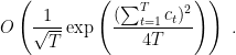
Note that this betting strategy could also be used in the OCO reduction. Given that we removed the logarithmic term in the exponent, in the 1-dimensional case, we would obtain a regret of

$\displaystyle \text{Regret}_T(u) \leq O\left(|u|\sqrt{T \ln \left(\frac{|u|\sqrt{T}}{\epsilon}+1\right)+\epsilon}\right),$

where we gained in the ${\sqrt{T}}$ term inside the logarithmic, instead of the ${T}$ term of the KT algorithm. This implies that now we can set ${\epsilon}$ to ${\sqrt{T}}$ and obtain an asymptotic rate of ${O(\sqrt{T})}$ rather than ${O(\sqrt{T \ln T})}$ .

3. History Bits

The first parameter-free algorithm for experts is from (Chaudhuri, K. and Freund, Y. and Hsu, D. J., 2009), named NormalHedge, where they obtained a bound similar to the one in (9) but with an additional ${\ln \ln T}$ term. Then, (Chernov, A. and Vovk, V., 2010) removed the log factors with an update without a closed form. (Orabona, F. and Pal, D., 2016) showed that this guarantee can be efficiently obtained through the novel reduction to coin-betting in Theorem 1. Later, these kind of regret guarantees were improved to depend on the sum of the squared losses rather than on time, but with an additional ${\ln \ln T}$ factor, in the Squint algorithm (Koolen, W. M. and van Erven, T., 2015). It is worth noting that the Squint algorithm can be interpreted exactly as a coin-betting algorithm plus the reduction in Theorem 1.

The betting strategy in (6) and (7) are new, and derived from the shifted-KT potentials in (Orabona, F. and Pal, D., 2016). The guarantee is the same obtained by the shifted-KT potentials, but the analysis can be done without knowing the properties of the gamma function.

4. Exercises

Exercise 1 Using the same proof technique in the lecture, find a betting strategy whose wealth depends on ${\sum_{t=1}^T |c_t|}$ rather than on ${T}$ .

6 Comments

Nicolò Campolongo says:

December 4, 2019 at 12:21 PM

Nice, post! The amount of work to remove just a ln T factor is impressive!
I have few questions: since you mentioned Squint, can you elaborate more on how it can be seen as a coin betting algorithm? I find Squint really appealing, since the sum of square losses should always be no worse than T, but it can actually be much better, for example it implies constant regret in a stochastic setting (see for example thm. 11 in http://proceedings.mlr.press/v35/gaillard14.pdf). Is it possible to give such bounds, or first-order bounds using a KT strategy?
Also, there should be some applications where the knowledge of the time horizon is not available in advance. For example, in the construction used to get strongly-adaptive regret bounds (as in your paper http://proceedings.mlr.press/v54/jun17a/jun17a.pdf), I guess in this case it would be better to use Squint?

Thank you!

LikeLike

1. Nicolò Campolongo says:
  
  December 4, 2019 at 12:31 PM
  
  Sorry, regarding the strongly-adaptive construction I suppose the real problem is not the knowledge of T but the fact that you shouldn’t be able to use a doubling trick.
  
  Nicolò
  
  LikeLike
  
bremen79 says:

December 5, 2019 at 9:51 PM

The main difficulty in dealing with Squint is the “improper prior” they use. The rest is easy: by induction you can show that any potential of the form used by Squint gives a lower bound to the wealth. I will try to find the time to write a post on it: it is easier to explain with equations.
If you don’t care about improper prior, you would get additional log factors. Note that Squint gets a log log term that is probably unavoidable.

In alternative, if you just care about the constant regret in the stochastic setting, you can get it easily with a strategy that depends on sum |c_i| rather than sum c_i^2. This is much easier to do and it was done in OCO with Pistol (https://arxiv.org/abs/1406.3816) and Learning with Experts with AdaNormalHedge (http://proceedings.mlr.press/v40/Luo15.pdf). Note that again it can be proven that these are betting algorithms. The only difference is that they bet with the lower bound to the wealth times the betting fraction rather than using the actual wealth times the betting fraction. Note that the proof of AdaNormalHedge is complex only because they truncate negative predictions inside the potential rather than outside as in equation (3). If you remove the truncation, the proof becomes easy.

Trying to adapt directly KT to obtain this kind of guarantees is not a good idea: you quickly loose the closed form expression. Indeed, KT is nothing else than FTRL with certain losses and a certain regularizer. You can use the same FTRL strategy if the coin is “continuous”, but you don’t have a closed form anymore.

LikeLike

Nicolò Campolongo says:

December 7, 2019 at 10:11 AM

Cool, thanks! You are probably already aware of it but there’s also a “dual” view of KT for experts from an exponential weights point of view in http://proceedings.mlr.press/v75/hoeven18a/hoeven18a.pdf

LikeLiked by 1 person

Yichi Zhou says:

December 13, 2021 at 4:05 AM

Nice post! Your work on parameter-free online learning is rather impressive! I’m curious if it is possible to develop parameter-free version of accelerated gradient descent as well?

LikeLiked by 1 person

1. bremen79 says:
  
  December 13, 2021 at 6:39 AM
  
  Hi Yichi, thanks for your question!
  The key point is that accelerated algorithms makes sense for smooth functions, while parameter-free algorithms make sense for non-smooth ones. In fact, with a non-smooth function the (sub)-gradient does not give any information on how far is the optimum and the setting of the learning rate becomes critical. Instead, in the smooth world the gradients are very informative and knowledge of the smoothness constant allows to easily optimally set the learning rate. Hence, we should first define what we mean by “parameter-free” for smooth optimization. Also, it is relatively easy to estimate smoothness. Indeed, the accelerated algorithm FISTA (https://www.math.mcgill.ca/yyang/comp/papers/FISTA.pdf) has a line-search procedure that essentially estimates the smoothness parameter. It is still non-trivial to estimate the smoothness constant in the stochastic setting, but definitely doable.
  A different but related result you might be interested is that parameter-free algorithms allow you to adapt to the strong convexity (that is harder to estimate than smoothness), see section 6 in https://arxiv.org/pdf/1802.06293.pdf
  
  LikeLike
  
Pingback: Saddle-Points, Game Theory, and Boosting – Parameter-free Learning and Optimization Algorithms