This time I will describe an online algorithm that is better than the Percetron algorithm. This is one of those results that I consider fundamental in online learning, yet not enough widely known.
1. The Gaptron Algorithm
We introduce the Gaptron algorithm, a randomized first-order algorithm for online binary and multiclass classification. The key motivation behind Gaptron is to exploit the surrogate gap, which is the difference between the true zero-one loss and the convex surrogate loss function used for optimization. Standard analyses of online learning algorithms often bound the regret with respect to the surrogate loss. However, this can be a loose upper bound on the actual number of mistakes. The Gaptron algorithm is designed to tighten this analysis by actively managing the surrogate gap, leading to better mistake bounds. For didactical reasons, in the following we will focus on the binary version of the Gaptron algorithm.
The algorithm maintains a weight vector 


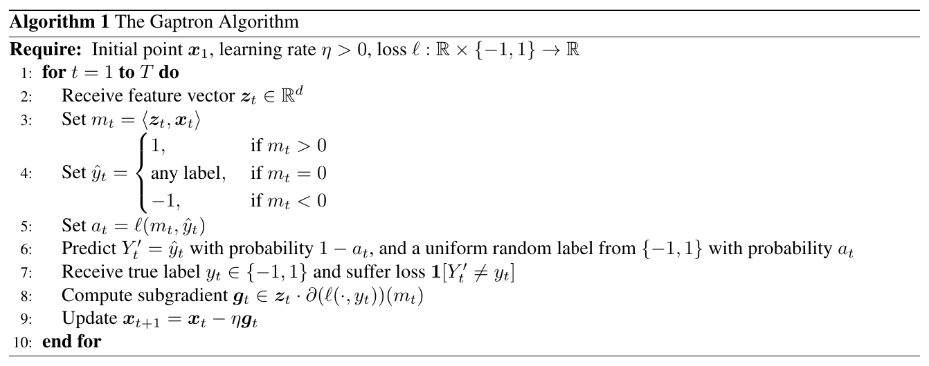
We now present a theorem on the expected number of mistakes for the Gaptron algorithm when using self-bounded losses, a weaker assumption than smoothness for convex functions.
Definition 1 (Self-bounded Function). Let
bounded from below, and subdifferentiable in a set
. We say that
is
-self-bounded in
if

Remark 1. Self-bounded functions are also convex in
Clearly, a convex
Example 1. Let
defined as
. The function
, hence it is not smooth. However, it is easy to verify that it is
-self-bounded.
Theorem 1. Let
where
. Assume that
is
for all
;
for
;
and
.
Let
for all
. Set the learning rate
and the gap map
. Then, the expected number of mistakes of the Gaptron algorithm (Algorithm 1) is upper bounded as
![\displaystyle \mathop{\mathbb E}\left[\sum_{t=1}^T \boldsymbol{1}[Y'_t \neq y_t]\right] \leq \sum_{t=1}^T \ell_t({\boldsymbol u}) + \frac{\|{\boldsymbol u}-{\boldsymbol x}_1\|_2^2}{2\eta}, \qquad \forall {\boldsymbol u} \in {\mathbb R}^d~.](https://s0.wp.com/latex.php?latex=%5Cdisplaystyle+%5Cmathop%7B%5Cmathbb+E%7D%5Cleft%5B%5Csum_%7Bt%3D1%7D%5ET+%5Cboldsymbol%7B1%7D%5BY%27_t+%5Cneq+y_t%5D%5Cright%5D+%5Cleq+%5Csum_%7Bt%3D1%7D%5ET+%5Cell_t%28%7B%5Cboldsymbol+u%7D%29+%2B+%5Cfrac%7B%5C%7C%7B%5Cboldsymbol+u%7D-%7B%5Cboldsymbol+x%7D_1%5C%7C_2%5E2%7D%7B2%5Ceta%7D%2C+%5Cqquad+%5Cforall+%7B%5Cboldsymbol+u%7D+%5Cin+%7B%5Cmathbb+R%7D%5Ed%7E.+&bg=ffffff&fg=000000&s=0&c=20201002)
Proof: Using the fact that self-boundedness implies convexity, the analysis starts from the standard regret bound for Online Subgradient Descent (OSD), which for any 

The expected number of mistakes in round 
![\displaystyle \mathop{\mathbb E}_t[\boldsymbol{1}[Y'_t \neq y_t]] = (1-a_t)\boldsymbol{1}[\hat{y}_t \neq y_t] + \frac{a_t}{2}~.](https://s0.wp.com/latex.php?latex=%5Cdisplaystyle+%5Cmathop%7B%5Cmathbb+E%7D_t%5B%5Cboldsymbol%7B1%7D%5BY%27_t+%5Cneq+y_t%5D%5D+%3D+%281-a_t%29%5Cboldsymbol%7B1%7D%5B%5Chat%7By%7D_t+%5Cneq+y_t%5D+%2B+%5Cfrac%7Ba_t%7D%7B2%7D%7E.+&bg=ffffff&fg=000000&s=0&c=20201002)
Hence, we have
![\displaystyle \begin{aligned} \sum_{t=1}^T \mathop{\mathbb E}[\boldsymbol{1}[Y'_t \neq y_t]] -\sum_{t=1}^T \ell_t({\boldsymbol u}) &= \sum_{t=1}^T \mathop{\mathbb E}[\boldsymbol{1}[Y'_t \neq y_t]] - \sum_{t=1}^T \ell_t({\boldsymbol x}_t) + \sum_{t=1}^T \ell_t({\boldsymbol x}_t)-\sum_{t=1}^T \ell_t({\boldsymbol u})\\ &\leq \frac{\|{\boldsymbol u}-{\boldsymbol x}_1\|_2^2}{2\eta} + \sum_{t=1}^T \mathop{\mathbb E}\left[\boldsymbol{1}[Y'_t \neq y_t]-\ell_t({\boldsymbol x}_t) +\frac{\eta}{2} \|{\boldsymbol g}_t\|_2^2\right]\\ &= \frac{\|{\boldsymbol u}-{\boldsymbol x}_1\|_2^2}{2\eta} + \sum_{t=1}^T \mathop{\mathbb E}\left[(1-a_t)\boldsymbol{1}[\hat{y}_t \neq y_t] + \frac{a_t}{2}-\ell_t({\boldsymbol x}_t) +\frac{\eta}{2} \|{\boldsymbol g}_t\|_2^2\right]~. \end{aligned}](https://s0.wp.com/latex.php?latex=%5Cdisplaystyle+%5Cbegin%7Baligned%7D+%5Csum_%7Bt%3D1%7D%5ET+%5Cmathop%7B%5Cmathbb+E%7D%5B%5Cboldsymbol%7B1%7D%5BY%27_t+%5Cneq+y_t%5D%5D+-%5Csum_%7Bt%3D1%7D%5ET+%5Cell_t%28%7B%5Cboldsymbol+u%7D%29+%26%3D+%5Csum_%7Bt%3D1%7D%5ET+%5Cmathop%7B%5Cmathbb+E%7D%5B%5Cboldsymbol%7B1%7D%5BY%27_t+%5Cneq+y_t%5D%5D+-+%5Csum_%7Bt%3D1%7D%5ET+%5Cell_t%28%7B%5Cboldsymbol+x%7D_t%29+%2B+%5Csum_%7Bt%3D1%7D%5ET+%5Cell_t%28%7B%5Cboldsymbol+x%7D_t%29-%5Csum_%7Bt%3D1%7D%5ET+%5Cell_t%28%7B%5Cboldsymbol+u%7D%29%5C%5C+%26%5Cleq+%5Cfrac%7B%5C%7C%7B%5Cboldsymbol+u%7D-%7B%5Cboldsymbol+x%7D_1%5C%7C_2%5E2%7D%7B2%5Ceta%7D+%2B+%5Csum_%7Bt%3D1%7D%5ET+%5Cmathop%7B%5Cmathbb+E%7D%5Cleft%5B%5Cboldsymbol%7B1%7D%5BY%27_t+%5Cneq+y_t%5D-%5Cell_t%28%7B%5Cboldsymbol+x%7D_t%29+%2B%5Cfrac%7B%5Ceta%7D%7B2%7D+%5C%7C%7B%5Cboldsymbol+g%7D_t%5C%7C_2%5E2%5Cright%5D%5C%5C+%26%3D+%5Cfrac%7B%5C%7C%7B%5Cboldsymbol+u%7D-%7B%5Cboldsymbol+x%7D_1%5C%7C_2%5E2%7D%7B2%5Ceta%7D+%2B+%5Csum_%7Bt%3D1%7D%5ET+%5Cmathop%7B%5Cmathbb+E%7D%5Cleft%5B%281-a_t%29%5Cboldsymbol%7B1%7D%5B%5Chat%7By%7D_t+%5Cneq+y_t%5D+%2B+%5Cfrac%7Ba_t%7D%7B2%7D-%5Cell_t%28%7B%5Cboldsymbol+x%7D_t%29+%2B%5Cfrac%7B%5Ceta%7D%7B2%7D+%5C%7C%7B%5Cboldsymbol+g%7D_t%5C%7C_2%5E2%5Cright%5D%7E.+%5Cend%7Baligned%7D&bg=ffffff&fg=000000&s=0&c=20201002)
Let’s analyze the term we call the surrogate gap:
![\displaystyle \gamma_t = (1-a_t)\boldsymbol{1}[\hat{y}_t \neq y_t] + \frac{a_t}{2} - \ell_t({\boldsymbol x}_t) + \frac{\eta}{2}\|{\boldsymbol g}_t\|_2^2~.](https://s0.wp.com/latex.php?latex=%5Cdisplaystyle+%5Cgamma_t+%3D+%281-a_t%29%5Cboldsymbol%7B1%7D%5B%5Chat%7By%7D_t+%5Cneq+y_t%5D+%2B+%5Cfrac%7Ba_t%7D%7B2%7D+-+%5Cell_t%28%7B%5Cboldsymbol+x%7D_t%29+%2B+%5Cfrac%7B%5Ceta%7D%7B2%7D%5C%7C%7B%5Cboldsymbol+g%7D_t%5C%7C_2%5E2%7E.+&bg=ffffff&fg=000000&s=0&c=20201002)
The theorem is proven if we can show that 

The bound on the norm of the subgradient can be calculated through the self-boundedness of

Hence, we have two cases.
Case 
![\displaystyle \begin{aligned} \gamma_t &=(1-a_t)\boldsymbol{1}[\hat{y}_t \neq y_t] + \frac{a_t}{2} - \ell_t({\boldsymbol x}_t) + \frac{\eta}{2}\|{\boldsymbol g}_t\|_2^2\\ &\leq 1-\ell(m_t, \hat{y}_t) + \frac12 \ell(m_t, \hat{y}_t) - \ell(m_t, y_t) + \eta s R^2 \ell(m_t,y_t)\\ &= 1-\frac12 \ell(m_t, \hat{y}_t) - \frac12 \ell(m_t, y_t) - \frac12 \ell(m_t, y_t) + \eta s R^2 \ell(m_t, y_t)\\ &\leq - \frac12 \ell(m_t, y_t) + \eta s R^2 \ell(m_t, y_t), \end{aligned}](https://s0.wp.com/latex.php?latex=%5Cdisplaystyle+%5Cbegin%7Baligned%7D+%5Cgamma_t+%26%3D%281-a_t%29%5Cboldsymbol%7B1%7D%5B%5Chat%7By%7D_t+%5Cneq+y_t%5D+%2B+%5Cfrac%7Ba_t%7D%7B2%7D+-+%5Cell_t%28%7B%5Cboldsymbol+x%7D_t%29+%2B+%5Cfrac%7B%5Ceta%7D%7B2%7D%5C%7C%7B%5Cboldsymbol+g%7D_t%5C%7C_2%5E2%5C%5C+%26%5Cleq+1-%5Cell%28m_t%2C+%5Chat%7By%7D_t%29+%2B+%5Cfrac12+%5Cell%28m_t%2C+%5Chat%7By%7D_t%29+-+%5Cell%28m_t%2C+y_t%29+%2B+%5Ceta+s+R%5E2+%5Cell%28m_t%2Cy_t%29%5C%5C+%26%3D+1-%5Cfrac12+%5Cell%28m_t%2C+%5Chat%7By%7D_t%29+-+%5Cfrac12+%5Cell%28m_t%2C+y_t%29+-+%5Cfrac12+%5Cell%28m_t%2C+y_t%29+%2B+%5Ceta+s+R%5E2+%5Cell%28m_t%2C+y_t%29%5C%5C+%26%5Cleq+-+%5Cfrac12+%5Cell%28m_t%2C+y_t%29+%2B+%5Ceta+s+R%5E2+%5Cell%28m_t%2C+y_t%29%2C+%5Cend%7Baligned%7D&bg=ffffff&fg=000000&s=0&c=20201002)
where in the second inequality we used the assumption on the loss. Hence, we need 
Case 
![\displaystyle \begin{aligned} \gamma_t &=(1-a_t)\boldsymbol{1}[\hat{y}_t \neq y_t] + \frac{a_t}{2} - \ell_t({\boldsymbol x}_t) + \frac{\eta}{2}\|{\boldsymbol g}_t\|_2^2\\ &\leq \frac12 \ell(m_t, \hat{y}_t) - \ell(m_t, y_t) + \eta s R^2 \ell(m_t, y_t)\\ &= -\frac12 \ell(m_t, y_t) + \eta s R^2 \ell(m_t, y_t)~. \end{aligned}](https://s0.wp.com/latex.php?latex=%5Cdisplaystyle+%5Cbegin%7Baligned%7D+%5Cgamma_t+%26%3D%281-a_t%29%5Cboldsymbol%7B1%7D%5B%5Chat%7By%7D_t+%5Cneq+y_t%5D+%2B+%5Cfrac%7Ba_t%7D%7B2%7D+-+%5Cell_t%28%7B%5Cboldsymbol+x%7D_t%29+%2B+%5Cfrac%7B%5Ceta%7D%7B2%7D%5C%7C%7B%5Cboldsymbol+g%7D_t%5C%7C_2%5E2%5C%5C+%26%5Cleq+%5Cfrac12+%5Cell%28m_t%2C+%5Chat%7By%7D_t%29+-+%5Cell%28m_t%2C+y_t%29+%2B+%5Ceta+s+R%5E2+%5Cell%28m_t%2C+y_t%29%5C%5C+%26%3D+-%5Cfrac12+%5Cell%28m_t%2C+y_t%29+%2B+%5Ceta+s+R%5E2+%5Cell%28m_t%2C+y_t%29%7E.+%5Cend%7Baligned%7D&bg=ffffff&fg=000000&s=0&c=20201002)
Hence, again we need

Surprisingly, the use of the randomization allows to obtain a constant regret with respect to the cumulative loss of any comparator.
Remark 2. Observe that if
for some convex function
, then
implies the condition
We now show some examples of binary classification losses that satisfy the assumptions of the theorem.
Example 2. Consider the hinge loss, defined as
We will use the squared hinge loss,
that satisfies all the assumptions in Theorem 1 and it is
-self-bounded in its first argument. Hence, we have that the Gaptron using the squared hinge loss and
satisfies
So, if the problem is not linearly separable, we can greatly beat (in expectation) the bound on the number of mistakes we gave for the Perceptron in terms of the squared hinge loss.
An even better choice is the smoothed hinge loss:
This loss is always less than or equal to the squared hinge loss, it still satisfies all the assumptions of Theorem 1, and it is

![\displaystyle \mathop{\mathbb E}\left[\sum_{t=1}^T \boldsymbol{1}[Y'_t \neq y_t]\right] \leq \sum_{t=1}^T (\ell^\text{hinge}_t)^2({\boldsymbol u}) + 2\|{\boldsymbol u}-{\boldsymbol x}_1\|_2^2 R^2, \qquad \forall {\boldsymbol u} \in {\mathbb R}^d~.](https://s0.wp.com/latex.php?latex=%5Cdisplaystyle+%5Cmathop%7B%5Cmathbb+E%7D%5Cleft%5B%5Csum_%7Bt%3D1%7D%5ET+%5Cboldsymbol%7B1%7D%5BY%27_t+%5Cneq+y_t%5D%5Cright%5D+%5Cleq+%5Csum_%7Bt%3D1%7D%5ET+%28%5Cell%5E%5Ctext%7Bhinge%7D_t%29%5E2%28%7B%5Cboldsymbol+u%7D%29+%2B+2%5C%7C%7B%5Cboldsymbol+u%7D-%7B%5Cboldsymbol+x%7D_1%5C%7C_2%5E2+R%5E2%2C+%5Cqquad+%5Cforall+%7B%5Cboldsymbol+u%7D+%5Cin+%7B%5Cmathbb+R%7D%5Ed%7E.+&bg=ffffff&fg=000000&s=0&c=20201002)

Example 3. One can also use loss functions that give different weights to the errors of the two classes. For example, we can use the following function
where
and
. This loss penalizes more the errors on class 1. In this case, the loss function is
-self-bounded (but it is not smooth!) and it still satisfies the assumptions of Theorem 1.

2. History Bits
The Gaptron was introduced in van der Hoeven (2020), in turn based on some of the ideas in Neu&Zhivotovskiy (2020). He also described a multiclass variant for different surrogate losses, as well as a bandit variant. The proof here and the conditions in Theorem 1 were developed in collaboration with Dirk van der Hoeven, and he was so kind to allow me to reproduce them here.
More recently, Sakaue et al. (2024) extended the Gaptron algorithm to the structured prediction case, while Sakaue et al. (2025) extended it to the dynamic setting.
Acknowledgments
Thanks to Dirk van der Hoeven for the help in writing a short and general proof, and to Abed Razawy and Valentina Masarotto for feedback and comments.
Exercises
Exercise 1. Use FTRL with an increasing regularizer instead of OSD in the Gaptron to get rid of the need to know
to set the learning rate, , while still allowing unbounded feasible sets. Note that we make use of the knowledge of
