This post is part of the lecture notes of my class “Introduction to Online Learning” at Boston University, Fall 2019. I will publish two lectures per week.
You can find the lectures I published till now here.
Imagine the following repeated game:
In each round
- An adversary choose a real number in
and he keeps it secret
- You try to guess its real number, choosing
- The adversary’s number is revealed and you pay the squared difference
![{x_t \in [0,1]}](https://s0.wp.com/latex.php?latex=%7Bx_t+%5Cin+%5B0%2C1%5D%7D&bg=ffffff&fg=000000&s=0&c=20201002)

Basically, we want to guess a sequence of numbers as precisely as possible. To be a game, we now have to decide what is the “winning condition”. Let’s see what makes sense to consider as winning condition.
First, let’s simplify a bit the game. Let’s assume that the adversary is drawing the numbers i.i.d. from some fixed distribution over ![{[0,1]}](https://s0.wp.com/latex.php?latex=%7B%5B0%2C1%5D%7D&bg=ffffff&fg=000000&s=0&c=20201002)


![\displaystyle \label{eq:stoch_regret} \mathop{\mathbb E}_Y\left[\sum_{t=1}^T (x_t - Y)^2\right] - \sigma^2 T \ \ \ \ \ (1)](https://s0.wp.com/latex.php?latex=%5Cdisplaystyle+%5Clabel%7Beq%3Astoch_regret%7D+%5Cmathop%7B%5Cmathbb+E%7D_Y%5Cleft%5B%5Csum_%7Bt%3D1%7D%5ET+%28x_t+-+Y%29%5E2%5Cright%5D+-+%5Csigma%5E2+T+%5C+%5C+%5C+%5C+%5C+%281%29&bg=ffffff&fg=000000&s=0&c=20201002)
or equivalently considering the average
![\displaystyle \label{eq:av_stoch_regret} \frac{1}{T}\mathop{\mathbb E}_Y\left[\sum_{t=1}^T (x_t - Y)^2\right] - \sigma^2~. \ \ \ \ \ (2)](https://s0.wp.com/latex.php?latex=%5Cdisplaystyle+%5Clabel%7Beq%3Aav_stoch_regret%7D+%5Cfrac%7B1%7D%7BT%7D%5Cmathop%7B%5Cmathbb+E%7D_Y%5Cleft%5B%5Csum_%7Bt%3D1%7D%5ET+%28x_t+-+Y%29%5E2%5Cright%5D+-+%5Csigma%5E2%7E.+%5C+%5C+%5C+%5C+%5C+%282%29&bg=ffffff&fg=000000&s=0&c=20201002)
Clearly these quantities are positive and they seem to be a good measure, because they are somehow normalized with respect to the “difficulty” of the numbers generated by the adversary, through the variance of the distribution. It is not the only possible choice to measure our “success”, but for sure it is a reasonable one. It would make sense to consider a strategy “successful” if the difference in (1) grows sublinearly over time and equivalently if the difference in (2) goes to zero as the number of rounds 
Minimizing Regret. Given that we have converged to what it seems a good measure of success of the algorithm. Let’s now rewrite (1) in an equivalent way
![\displaystyle \mathop{\mathbb E}\left[\sum_{t=1}^T (x_t - Y)^2\right] - \min_{ x \in [0,1]} \ \mathop{\mathbb E}\left[\sum_{t=1}^T (x-Y)^2\right]~.](https://s0.wp.com/latex.php?latex=%5Cdisplaystyle+%5Cmathop%7B%5Cmathbb+E%7D%5Cleft%5B%5Csum_%7Bt%3D1%7D%5ET+%28x_t+-+Y%29%5E2%5Cright%5D+-+%5Cmin_%7B+x+%5Cin+%5B0%2C1%5D%7D+%5C+%5Cmathop%7B%5Cmathbb+E%7D%5Cleft%5B%5Csum_%7Bt%3D1%7D%5ET+%28x-Y%29%5E2%5Cright%5D%7E.+&bg=ffffff&fg=000000&s=0&c=20201002)
Now, the last step: remove the assumption on how the data is generated, just consider any arbitrary sequence of 
![\displaystyle \text{Regret}_T:=\sum_{t=1}^T (x_t - y_t)^2 - \min_{x \in [0,1]} \ \sum_{t=1}^T (x - y_t)^2](https://s0.wp.com/latex.php?latex=%5Cdisplaystyle+%5Ctext%7BRegret%7D_T%3A%3D%5Csum_%7Bt%3D1%7D%5ET+%28x_t+-+y_t%29%5E2+-+%5Cmin_%7Bx+%5Cin+%5B0%2C1%5D%7D+%5C+%5Csum_%7Bt%3D1%7D%5ET+%28x+-+y_t%29%5E2+&bg=ffffff&fg=000000&s=0&c=20201002)
grows sublinearly with 
Let’s generalize it a bit more, considering that the algorithm outputs a vector in 


This framework is pretty powerful, and it allows to reformulate a bunch of different problems in machine learning and optimization as similar games. More in general, with the regret framework we can analyze situations in which the data are not i.i.d. from a distribution, yet I would like to guarantee that the algorithm is “learning” something. For example, online learning can be used to analyze
- Click prediction problems;
- Routing on a network;
- Convergence to equilibrium of repeated games.
It can also be used to analyze stochastic algorithms, e.g., Stochastic Gradient Descent, but the adversarial nature of the analysis might give you suboptimal results. For example, it can be used to analyze momentum algorithms, but the adversarial nature of the losses essentially forces you to prove a convergence guarantee that treats the momentum term as a vanishing disturbance that does not help the algorithm in any way.
Let’s now go back to our number guessing game and let’s try a strategy to win it. Of course, this is one of the simplest example of online learning, without a real application. Yet, going through it we will uncover most of the key ingredients in online learning algorithms and their analysis.
A Winning Strategy. Can we win the number guessing name game? Note that we didn’t assume anything on how the adversary is deciding the numbers. In fact, the numbers can be generated in any way, even in an adaptive way based on our strategy. Indeed, they can be chosen adversarially, that is explicitly trying to make us lose the game. This is why we call the mechanism generating the number the adversary.
The fact that the numbers are adversarially chosen means that we can immediately rule out any strategy based on some statistical modelling on the data. In fact, it cannot work because the moment we estimate something and act on our estimate, the adversary can immediately change the way he is generating the data, ruining us. So, we have to think about something else. Yet, many times online learning algorithms will look like classic ones from statistical estimation, even if they work for different reasons.
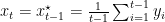
Now, let’s try to design a strategy to make the regret provably sublinear in time, regardless of how the adversary chooses the numbers. The first thing to do is to take a look at the best strategy in hindsight, that is argmin of the second term of the regret. It should be immediate to see that
![\displaystyle x^\star_T := \mathop{\text{argmin}}_{x \in [0,1]} \sum_{t=1}^T (x - y_t)^2 = \frac{1}{T} \sum_{t=1}^T y_t~.](https://s0.wp.com/latex.php?latex=%5Cdisplaystyle+x%5E%5Cstar_T+%3A%3D+%5Cmathop%7B%5Ctext%7Bargmin%7D%7D_%7Bx+%5Cin+%5B0%2C1%5D%7D+%5Csum_%7Bt%3D1%7D%5ET+%28x+-+y_t%29%5E2+%3D+%5Cfrac%7B1%7D%7BT%7D+%5Csum_%7Bt%3D1%7D%5ET+y_t%7E.+&bg=ffffff&fg=000000&s=0&c=20201002)
Now, given that we don’t know the future, for sure we cannot use 
Hence, on each round 
Let’s now try to show that indeed this strategy will allow us to win the game. We will use first principles and later introduce general proof methods. First, we will need a small lemma.
Lemma 1 Let
an arbitrary sequence of loss functions. Denote by
a minimizer of the cumulative losses over the previous

Proof: We prove it by induction over

that is trivially true. Now, for 
This inequality is equivalent to

where we removed the last element of the sums because they are the same. Now observe that

by induction hypothesis, and
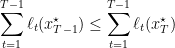
because 

Basically, the above lemma quantifies the idea the knowing the future and being adaptive to it is typically better than not being adaptive to it.
With this lemma, we can now prove that the regret will grow sublinearly, it particular it will be logarithmic in time. Note that we will not prove that our strategy is minimax optimal, even if it is possible to show that the logarithmic dependency on time is unavoidable for this problem.
Theorem 2 Let
an arbitrary sequence of numbers. Let the algorithm’s output
. Then, we have
![\displaystyle \text{Regret}_T = \sum_{t=1}^T (x_t - y_t)^2 - \min_{x \in [0,1]} \ \sum_{t=1}^T (x - y_t)^2 \leq 4 + 4\ln T~.](https://s0.wp.com/latex.php?latex=%5Cdisplaystyle+%5Ctext%7BRegret%7D_T+%3D+%5Csum_%7Bt%3D1%7D%5ET+%28x_t+-+y_t%29%5E2+-+%5Cmin_%7Bx+%5Cin+%5B0%2C1%5D%7D+%5C+%5Csum_%7Bt%3D1%7D%5ET+%28x+-+y_t%29%5E2+%5Cleq+4+%2B+4%5Cln+T%7E.+&bg=ffffff&fg=000000&s=0&c=20201002)
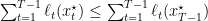
Proof: We use Lemma 1 to upper bound the regret:
![\displaystyle \begin{aligned} \sum_{t=1}^T (x_t - y_t)^2 - \min_{x \in [0,1]} \ \sum_{t=1}^T (x - y_t)^2 = \sum_{t=1}^T (x^\star_{t-1} - y_t)^2 - \sum_{t=1}^T (x^\star_T - y_t)^2 \leq \sum_{t=1}^T (x^\star_{t-1} - y_t)^2 - \sum_{t=1}^T (x^\star_t - y_t)^2~. \end{aligned}](https://s0.wp.com/latex.php?latex=%5Cdisplaystyle+%5Cbegin%7Baligned%7D+%5Csum_%7Bt%3D1%7D%5ET+%28x_t+-+y_t%29%5E2+-+%5Cmin_%7Bx+%5Cin+%5B0%2C1%5D%7D+%5C+%5Csum_%7Bt%3D1%7D%5ET+%28x+-+y_t%29%5E2+%3D+%5Csum_%7Bt%3D1%7D%5ET+%28x%5E%5Cstar_%7Bt-1%7D+-+y_t%29%5E2+-+%5Csum_%7Bt%3D1%7D%5ET+%28x%5E%5Cstar_T+-+y_t%29%5E2+%5Cleq+%5Csum_%7Bt%3D1%7D%5ET+%28x%5E%5Cstar_%7Bt-1%7D+-+y_t%29%5E2+-+%5Csum_%7Bt%3D1%7D%5ET+%28x%5E%5Cstar_t+-+y_t%29%5E2%7E.+%5Cend%7Baligned%7D&bg=ffffff&fg=000000&s=0&c=20201002)
Now, let’s take a look at each difference in the sum in the last equation. We have that
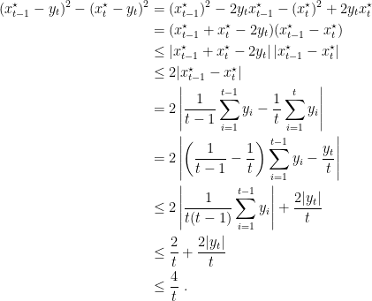
Hence, overall we have
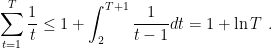
![\displaystyle \sum_{t=1}^T (x_t - y_t)^2 - \min_{x \in [0,1]} \ \sum_{t=1}^T (x - y_t)^2 \leq 4\sum_{t=1}^T\frac{1}{t}~.](https://s0.wp.com/latex.php?latex=%5Cdisplaystyle+%5Csum_%7Bt%3D1%7D%5ET+%28x_t+-+y_t%29%5E2+-+%5Cmin_%7Bx+%5Cin+%5B0%2C1%5D%7D+%5C+%5Csum_%7Bt%3D1%7D%5ET+%28x+-+y_t%29%5E2+%5Cleq+4%5Csum_%7Bt%3D1%7D%5ET%5Cfrac%7B1%7D%7Bt%7D%7E.+&bg=ffffff&fg=000000&s=0&c=20201002)

For the upper bound the last sum, observe that we are trying to find an upper bound to the green area in Figure 1. As you can see from the picture, it can be upper bounded by 1 plus the integral of 


There are few of things to stress on this strategy. The strategy does not have parameters to tune (e.g. learning rates, regularizers). Note that the presence of parameters does not make sense in online learning: We have only one stream of data and we cannot run our algorithm over it multiple times to select the best parameter! Also, it does not need to maintain a complete record of the past, but only a “summary” of it, through the running average. This gives a computationally efficient algorithm. When we design online learning algorithms, we will strive to achieve all these characteristics. Last thing that I want to stress is that the algorithm does not use gradients: Gradients are useful and we will use them a lot, but they don’t constitute the entire world of online optimization.
Before going on I want to remind you that, as seen above, this is different from the classic setting in statistical machine learning. So, for example, “overfitting” has absolutely no meaning here. Same for “generalization gap” and similar ideas linked to a training/testing scenario.
In the next lectures, we will introduce our first algorithm for online optimization for convex losses: Online Gradient Descent.
Exercises
Exercise 1 Extend the previous algorithm and analysis to the case when the adversary selects a vector
such that
, the algorithm guesses a vector
, and the loss function is
. Show an upper bound to the regret that is logarithmic in
.

Hi, thanks for the blog.
Is it an argmin in the definition of x_{*}^{T} ?
LikeLike
Yes, thanks! Fixed
LikeLike
Hello, in the definition of regret is there a missing subscript t for the first loss, i.e. \ell ({\boldsymbol x}_t) instead of \ell_t ({\boldsymbol x}_t)?
“.. Regret over a sequence of loss functions with respect to an arbitrary competitor {{\boldsymbol u} \in V\subseteq {\mathbb R}^d}
\text{Regret}_T({\boldsymbol u}):=\sum_{t=1}^T \ell ({\boldsymbol x}_t) – \sum_{t=1}^T \ell_t({\boldsymbol u})~.
”
Regarding the exercise, is it true that the regret bound should be the same except for a factor of d, i.e. 4d (1 + \ln T)?
LikeLike
Thanks for finding the typo! Fixed.
Regarding the exercise, you should be able to prove a regret without dependency on , we will see how this week using strong convexity. The dependency on
  might appear if you try to solve the problem coordinate-wise. Instead, mirroring the proof we did using inner products and L2 norms you should get the right regret.
LikeLike
Thanks a lot for the writeup. Is the definition of regret in the non-stochastic case (i.e., the term in the fourth display, $Regret_T$) guaranteed to be non-negative?
LikeLike
No, it is not! Even if for many online learning problems it is possible to show that there exists a strategy for the adversary that guarantee a positive regret, no matter what the online algorithm does.
LikeLike
Hello, thanks for the blog. In the first line of the proof of Lemma 1, shouldn’t the base case be $\ell_1(x^\star_1) \leq \ell_1(x^\star_1)$ ?
LikeLike
Fixed, thanks!
LikeLike
Thanks for your writing! I notice that quantity (1) is non-negative but the $\mathrm{Regret}_T$ may be negative since the expectation is removed. Does it matter for Regret to take negative values?
LikeLike
This was already asked and answered, see above 🙂
Maybe I should add it to the text.
LikeLike
Hi there! small suggestion, the bounding of sum_overT(1/t) can also be shown using lemma 4.13, there is also an exercise in Chapter 2, 2.1, that can leverage it. Maybe showing that earlier would be beneficial.
Best,
Pedram
LikeLike
Hi Pedram, I know 🙂
I wanted the first chapter to be single and only using first principles for a couple of reasons:
1) in CS there is a tendency to explain online learning only from first principles. While I don’t like this teaching approach, I wanted at least at the beginning to follow a similar route.
2) The notes are meant to be read chapter by chapter, so I didn’t want to scare the people right away 🙂
But you are right that I might introduce that lemma earlier anyway.
LikeLike