In this post, I want to explain what we can show for Stochastic Gradient Descent (SGD) when used on non-convex smooth functions. The first results are known and very easy to obtain, the last one instead is a result by (Bertsekas and Tsitsiklis, 2000) that is not as known as it should be, maybe for their long proof. Some years ago, I found a way to distill their proof in a simple lemma that I present here.
1. SGD on Non-Convex Smooth Functions
We are interested in minimizing a smooth non-convex function 


![{\mathop{\mathbb E}_{\xi}[\|\nabla F({\boldsymbol x}) - g({\boldsymbol x},\xi)\|^2_2]\leq \sigma^2 <\infty}](https://s0.wp.com/latex.php?latex=%7B%5Cmathop%7B%5Cmathbb+E%7D_%7B%5Cxi%7D%5B%5C%7C%5Cnabla+F%28%7B%5Cboldsymbol+x%7D%29+-+g%28%7B%5Cboldsymbol+x%7D%2C%5Cxi%29%5C%7C%5E2_2%5D%5Cleq+%5Csigma%5E2+%3C%5Cinfty%7D&bg=ffffff&fg=000000&s=0&c=20201002)
Given that the function 


Last thing we will assume is that the function 
Hence, I start from a point 
where 
First, let’s see practically how SGD behaves w.r.t. Gradient Descent (GD) on the same problem.

 . In SGD the derivative is corrupted by additive Gaussian noise.
In Figure 1, we are minimizing 
Will 

This is more difficult to answer than what you might think. However, this is a basic question to know if it actually makes sense to run SGD for a bunch of iterations and return the last iterate, that is how 99% of the people use SGD on a non-convex problem.
To warm up, let’s first see what we can prove in a finite-time setting.
As all other similar analysis, we need to construct a potential (Lyapunov) function that allows us to analyze it. In the convex case, we would study 


In words, this means that a smooth function is always upper bounded by a quadratic function. Note that this property does not require convexity, so we can safely use it. Thanks to this property, let’s see how our potential evolves over time during the optimization of SGD.

Now, let’s denote by 


![\displaystyle \begin{aligned} \mathop{\mathbb E}_t[F({\boldsymbol x}_{t+1})] &\leq F({\boldsymbol x}_t) - \eta_t \|\nabla F({\boldsymbol x}_t)\|^2_2 + \frac{\eta_t^2 L}{2} \mathop{\mathbb E}_t \| g({\boldsymbol x}_t, \xi_t)\|^2_2 \\ &= F({\boldsymbol x}_t) - \eta_t \|\nabla F({\boldsymbol x}_t)\|^2_2 + \frac{\eta_t^2 L}{2} \mathop{\mathbb E}_t \|\nabla F({\boldsymbol x}_t) - g({\boldsymbol x}_t, \xi_t) - \nabla F({\boldsymbol x}_t)\|^2_2 \\ &= F({\boldsymbol x}_t) - \eta_t \|\nabla F({\boldsymbol x}_t)\|^2_2 + \frac{\eta_t^2 L}{2} \left(\mathop{\mathbb E}_t \|\nabla F({\boldsymbol x}_t) - g({\boldsymbol x}_t, \xi_t)\|^2_2 + \|\nabla F({\boldsymbol x}_t)\|^2_2\right) \\ &\leq F({\boldsymbol x}_t) - \left(\eta_t - \frac{\eta_t^2 L}{2}\right)\|\nabla F({\boldsymbol x}_t)\|^2_2 + \frac{\eta_t^2 L}{2} \sigma^2, \end{aligned}](https://s0.wp.com/latex.php?latex=%5Cdisplaystyle+%5Cbegin%7Baligned%7D+%5Cmathop%7B%5Cmathbb+E%7D_t%5BF%28%7B%5Cboldsymbol+x%7D_%7Bt%2B1%7D%29%5D+%26%5Cleq+F%28%7B%5Cboldsymbol+x%7D_t%29+-+%5Ceta_t+%5C%7C%5Cnabla+F%28%7B%5Cboldsymbol+x%7D_t%29%5C%7C%5E2_2+%2B+%5Cfrac%7B%5Ceta_t%5E2+L%7D%7B2%7D+%5Cmathop%7B%5Cmathbb+E%7D_t+%5C%7C+g%28%7B%5Cboldsymbol+x%7D_t%2C+%5Cxi_t%29%5C%7C%5E2_2+%5C%5C+%26%3D+F%28%7B%5Cboldsymbol+x%7D_t%29+-+%5Ceta_t+%5C%7C%5Cnabla+F%28%7B%5Cboldsymbol+x%7D_t%29%5C%7C%5E2_2+%2B+%5Cfrac%7B%5Ceta_t%5E2+L%7D%7B2%7D+%5Cmathop%7B%5Cmathbb+E%7D_t+%5C%7C%5Cnabla+F%28%7B%5Cboldsymbol+x%7D_t%29+-+g%28%7B%5Cboldsymbol+x%7D_t%2C+%5Cxi_t%29+-+%5Cnabla+F%28%7B%5Cboldsymbol+x%7D_t%29%5C%7C%5E2_2+%5C%5C+%26%3D+F%28%7B%5Cboldsymbol+x%7D_t%29+-+%5Ceta_t+%5C%7C%5Cnabla+F%28%7B%5Cboldsymbol+x%7D_t%29%5C%7C%5E2_2+%2B+%5Cfrac%7B%5Ceta_t%5E2+L%7D%7B2%7D+%5Cleft%28%5Cmathop%7B%5Cmathbb+E%7D_t+%5C%7C%5Cnabla+F%28%7B%5Cboldsymbol+x%7D_t%29+-+g%28%7B%5Cboldsymbol+x%7D_t%2C+%5Cxi_t%29%5C%7C%5E2_2+%2B+%5C%7C%5Cnabla+F%28%7B%5Cboldsymbol+x%7D_t%29%5C%7C%5E2_2%5Cright%29+%5C%5C+%26%5Cleq+F%28%7B%5Cboldsymbol+x%7D_t%29+-+%5Cleft%28%5Ceta_t+-+%5Cfrac%7B%5Ceta_t%5E2+L%7D%7B2%7D%5Cright%29%5C%7C%5Cnabla+F%28%7B%5Cboldsymbol+x%7D_t%29%5C%7C%5E2_2+%2B+%5Cfrac%7B%5Ceta_t%5E2+L%7D%7B2%7D+%5Csigma%5E2%2C+%5Cend%7Baligned%7D&bg=ffffff&fg=000000&s=0&c=20201002)
where in the inequality we have used the fact that the variance of the stochastic gradient is bounded by 
![\displaystyle \begin{aligned} \sum_{t=1}^T \left(\eta_t - \frac{\eta_t^2 L}{2}\right) \mathop{\mathbb E}[\|\nabla F({\boldsymbol x}_t)\|^2_2] &\leq \sum_{t=1}^T \left(\mathop{\mathbb E}[F({\boldsymbol x}_t)] - \mathop{\mathbb E}[F({\boldsymbol x}_{t+1})]\right) + \frac{\sigma^2 L}{2} \sum_{t=1}^T \eta_t^2 \\ &= F({\boldsymbol x}_1) - \mathop{\mathbb E}[F({\boldsymbol x}_{T+1})] + \frac{\sigma^2 L}{2} \sum_{t=1}^T \eta_t^2 \\ &\leq F({\boldsymbol x}_1) - F^\star + \frac{\sigma^2 L}{2} \sum_{t=1}^T \eta_t^2~. & (1) \\\end{aligned}](https://s0.wp.com/latex.php?latex=%5Cdisplaystyle+%5Cbegin%7Baligned%7D+%5Csum_%7Bt%3D1%7D%5ET+%5Cleft%28%5Ceta_t+-+%5Cfrac%7B%5Ceta_t%5E2+L%7D%7B2%7D%5Cright%29+%5Cmathop%7B%5Cmathbb+E%7D%5B%5C%7C%5Cnabla+F%28%7B%5Cboldsymbol+x%7D_t%29%5C%7C%5E2_2%5D+%26%5Cleq+%5Csum_%7Bt%3D1%7D%5ET+%5Cleft%28%5Cmathop%7B%5Cmathbb+E%7D%5BF%28%7B%5Cboldsymbol+x%7D_t%29%5D+-+%5Cmathop%7B%5Cmathbb+E%7D%5BF%28%7B%5Cboldsymbol+x%7D_%7Bt%2B1%7D%29%5D%5Cright%29+%2B+%5Cfrac%7B%5Csigma%5E2+L%7D%7B2%7D+%5Csum_%7Bt%3D1%7D%5ET+%5Ceta_t%5E2+%5C%5C+%26%3D+F%28%7B%5Cboldsymbol+x%7D_1%29+-+%5Cmathop%7B%5Cmathbb+E%7D%5BF%28%7B%5Cboldsymbol+x%7D_%7BT%2B1%7D%29%5D+%2B+%5Cfrac%7B%5Csigma%5E2+L%7D%7B2%7D+%5Csum_%7Bt%3D1%7D%5ET+%5Ceta_t%5E2+%5C%5C+%26%5Cleq+F%28%7B%5Cboldsymbol+x%7D_1%29+-+F%5E%5Cstar+%2B+%5Cfrac%7B%5Csigma%5E2+L%7D%7B2%7D+%5Csum_%7Bt%3D1%7D%5ET+%5Ceta_t%5E2%7E.+%26+%281%29+%5C%5C%5Cend%7Baligned%7D&bg=ffffff&fg=000000&s=0&c=20201002)
Let’s see how useful this inequality is: consider a constant step size 

![\displaystyle \begin{aligned} \frac{1}{T}\sum_{t=1}^T \mathop{\mathbb E}[\|\nabla F({\boldsymbol x}_t)\|^2_2] &\leq \frac{2(F({\boldsymbol x}_1) - F^\star)}{\eta_1 T} + \sigma^2 L \eta_1 \\ &= \frac{2(F({\boldsymbol x}_1) - F^\star)}{T}\max\left(L, \frac{\sigma \sqrt{T}}{\alpha}\right) + \sigma L \alpha \frac{1}{\sqrt{T}} \\ &\leq \frac{2(F({\boldsymbol x}_1) - F^\star)}{T}\left(L+\frac{\sigma \sqrt{T}}{\alpha}\right) + \sigma L \alpha \frac{1}{\sqrt{T}} \\ &= \frac{2 L (F({\boldsymbol x}_1) - F^\star)}{T} + \left(\frac{2 (F({\boldsymbol x}_1) - F^\star)}{ \alpha} + L \alpha\right) \frac{\sigma}{\sqrt{T}}~. \end{aligned}](https://s0.wp.com/latex.php?latex=%5Cdisplaystyle+%5Cbegin%7Baligned%7D+%5Cfrac%7B1%7D%7BT%7D%5Csum_%7Bt%3D1%7D%5ET+%5Cmathop%7B%5Cmathbb+E%7D%5B%5C%7C%5Cnabla+F%28%7B%5Cboldsymbol+x%7D_t%29%5C%7C%5E2_2%5D+%26%5Cleq+%5Cfrac%7B2%28F%28%7B%5Cboldsymbol+x%7D_1%29+-+F%5E%5Cstar%29%7D%7B%5Ceta_1+T%7D+%2B+%5Csigma%5E2+L+%5Ceta_1+%5C%5C+%26%3D+%5Cfrac%7B2%28F%28%7B%5Cboldsymbol+x%7D_1%29+-+F%5E%5Cstar%29%7D%7BT%7D%5Cmax%5Cleft%28L%2C+%5Cfrac%7B%5Csigma+%5Csqrt%7BT%7D%7D%7B%5Calpha%7D%5Cright%29+%2B+%5Csigma+L+%5Calpha+%5Cfrac%7B1%7D%7B%5Csqrt%7BT%7D%7D+%5C%5C+%26%5Cleq+%5Cfrac%7B2%28F%28%7B%5Cboldsymbol+x%7D_1%29+-+F%5E%5Cstar%29%7D%7BT%7D%5Cleft%28L%2B%5Cfrac%7B%5Csigma+%5Csqrt%7BT%7D%7D%7B%5Calpha%7D%5Cright%29+%2B+%5Csigma+L+%5Calpha+%5Cfrac%7B1%7D%7B%5Csqrt%7BT%7D%7D+%5C%5C+%26%3D+%5Cfrac%7B2+L+%28F%28%7B%5Cboldsymbol+x%7D_1%29+-+F%5E%5Cstar%29%7D%7BT%7D+%2B+%5Cleft%28%5Cfrac%7B2+%28F%28%7B%5Cboldsymbol+x%7D_1%29+-+F%5E%5Cstar%29%7D%7B+%5Calpha%7D+%2B+L+%5Calpha%5Cright%29+%5Cfrac%7B%5Csigma%7D%7B%5Csqrt%7BT%7D%7D%7E.+%5Cend%7Baligned%7D&bg=ffffff&fg=000000&s=0&c=20201002)
What we got is almost a convergence result: it says that the average of the norm of the gradients is going to zero as 

It is also interesting to see that the convergence rate has two terms: a fast rate 


2. The Magic Trick: Randomly Stopped SGD
The above reasoning is interesting but it is not a solution to our question: does the last iterate of SGD converge? Yes or no?
There is a possible work-around that looks like a magic trick. Let’s take one iterate of SGD uniformly at random among 

![\displaystyle \mathop{\mathbb E}[\|\nabla F({\boldsymbol x}_I)\|^2_2] = \frac{1}{T} \sum_{t=1}^T \mathop{\mathbb E}[\|\nabla F({\boldsymbol x}_t)\|^2_2] \leq \frac{2 L (F({\boldsymbol x}_1) - F^\star)}{T} + \left(\frac{2 (F({\boldsymbol x}_1) - F^\star)}{ \alpha} + L \alpha\right) \frac{\sigma}{\sqrt{T}}~.](https://s0.wp.com/latex.php?latex=%5Cdisplaystyle+%5Cmathop%7B%5Cmathbb+E%7D%5B%5C%7C%5Cnabla+F%28%7B%5Cboldsymbol+x%7D_I%29%5C%7C%5E2_2%5D+%3D+%5Cfrac%7B1%7D%7BT%7D+%5Csum_%7Bt%3D1%7D%5ET+%5Cmathop%7B%5Cmathbb+E%7D%5B%5C%7C%5Cnabla+F%28%7B%5Cboldsymbol+x%7D_t%29%5C%7C%5E2_2%5D+%5Cleq+%5Cfrac%7B2+L+%28F%28%7B%5Cboldsymbol+x%7D_1%29+-+F%5E%5Cstar%29%7D%7BT%7D+%2B+%5Cleft%28%5Cfrac%7B2+%28F%28%7B%5Cboldsymbol+x%7D_1%29+-+F%5E%5Cstar%29%7D%7B+%5Calpha%7D+%2B+L+%5Calpha%5Cright%29+%5Cfrac%7B%5Csigma%7D%7B%5Csqrt%7BT%7D%7D%7E.+&bg=ffffff&fg=000000&s=0&c=20201002)
Basically, it says that if run SGD for
This is a very important result and also a standard one in these days. It should be intuitive why the randomization helps: From Figure 1 it is clear that we might be unlucky in the last iteration of SGD, however randomizing in expectation we smooth out the noise and get a decreasing gradient. However, we just changed the target because we still didn’t prove if the last iterate converges. So, we need an alternative way.
3. The Disappointing Lim Inf
Let’s consider again (1). This time let’s select any time-varying positive stepsizes that satisfy
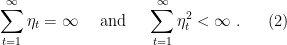
These two conditions are classic in the study of stochastic approximation. The first condition is needed to be able to travel arbitrarily far from the initial point, while the second one is needed to keep the variance of the noise under control. The classic learning rate of 

With such a choice, we get
![\displaystyle \sum_{t=1}^\infty \left(\eta_t - \frac{\eta_t^2 L}{2}\right) \mathop{\mathbb E}[\|\nabla F({\boldsymbol x}_t)\|^2_2] \leq F({\boldsymbol x}_1) - F^\star + \frac{\sigma^2 L}{2} \sum_{t=1}^\infty \eta_t^2 < \infty,](https://s0.wp.com/latex.php?latex=%5Cdisplaystyle+%5Csum_%7Bt%3D1%7D%5E%5Cinfty+%5Cleft%28%5Ceta_t+-+%5Cfrac%7B%5Ceta_t%5E2+L%7D%7B2%7D%5Cright%29+%5Cmathop%7B%5Cmathbb+E%7D%5B%5C%7C%5Cnabla+F%28%7B%5Cboldsymbol+x%7D_t%29%5C%7C%5E2_2%5D+%5Cleq+F%28%7B%5Cboldsymbol+x%7D_1%29+-+F%5E%5Cstar+%2B+%5Cfrac%7B%5Csigma%5E2+L%7D%7B2%7D+%5Csum_%7Bt%3D1%7D%5E%5Cinfty+%5Ceta_t%5E2+%3C+%5Cinfty%2C+&bg=ffffff&fg=000000&s=0&c=20201002)
where we have used the second condition in the inequality. Now, the condition 


![\displaystyle \sum_{t=T_L}^\infty \eta_t \mathop{\mathbb E}[\|\nabla F({\boldsymbol x}_t)\|^2_2] < \infty~.](https://s0.wp.com/latex.php?latex=%5Cdisplaystyle+%5Csum_%7Bt%3DT_L%7D%5E%5Cinfty+%5Ceta_t+%5Cmathop%7B%5Cmathbb+E%7D%5B%5C%7C%5Cnabla+F%28%7B%5Cboldsymbol+x%7D_t%29%5C%7C%5E2_2%5D+%3C+%5Cinfty%7E.+&bg=ffffff&fg=000000&s=0&c=20201002)
This implies that 


Wait, what? What is this 
This is very disappointing and we might be tempted to believe that this is the best that we can do. Fortunately, this is not the case. In fact, in a seminal paper (Bertsekas and Tsitsiklis, 2000) proved the convergence of the gradients of SGD to zero with probability 1 under very weak assumptions. Their proof is very convoluted also due to the assumptions they used, but in the following I’ll show a much simpler proof.
4. The Asymptotic Proof in Few Lines
In 2018, I found a way to get the same result of (Bertsekas and Tsitsiklis, 2000) distilling their long proof in the following Lemma, whose proof is in the Appendix. It turns out that this Lemma is essentially all what we need.
Lemma 1. Let
be two non-negative sequences and
a sequence of vectors in a vector space
. Let
and assume
and
. Assume also that there exists
such that
, where
is such that
. Then,
converges to 0.
We are now finally ready to prove the asymptotic convergence with probability 1.
Theorem 2. Assume that we use SGD on a
goes to zero with probability 1.
Proof: We want to use Lemma 1 on 
The assumptions and the reasoning above imply that, with probability 1, 


Overall, with probability 1 the assumptions of Lemma 1 are verified with 

We did it! Finally, we proved that the gradients of SGD do indeed converge to zero with probability 1. This means that with probability 1 for any 


Even if I didn’t actually use any intuition in crafting the above proof (I rarely use “intuition” to prove things), Yann Ollivier provided the following intuition for this proof: the proof is implicitly studying how far apart GD and SGD are. However, instead of estimating the distance between the two processes over a single update, it does it over large period of time through the term 
5. History Bits
The idea of taking one iterate at random in SGD was proposed in (Ghadimi and Lan, 2013) and it reminds me the well-known online-to-batch conversion through randomization. The conditions on the learning rates in (2) go back to (Robbins and Monro, 1951). (Bertsekas and Tsitsiklis, 2000) contains a good review of previous work on asymptotic convergence of SGD, while a recent paper on this topic is (Patel, V., 2020).
I derived Lemma 1 as an extension of Proposition 2 in (Alber et al., 1998)/Lemma A.5 in (Mairal, 2013). Studying the proof of (Bertsekas and Tsitsiklis, 2000), I realized that I could change (Alber et al., 1998, Proposition 2) into what I needed. I had this proof sitting in my unpublished notes for 2 years, so I decided to write a blog post on it.
My actual small contribution to this line of research is a lim inf convergence for SGD with AdaGrad stepsizes (Li and Orabona, 2019), but under stronger assumptions on the noise.
Note that the 20-30 years ago there were many papers studying the asymptotic convergence of SGD and its variants in various settings. Then, the taste of the community changed moving from asymptotic convergence to finite-time rates. As it often happens when a new trend takes over the previous one, new generations tend to be oblivious to the old results and proof techniques. The common motivation to ignore these past results is that the finite-time analysis is superior to the asymptotic one, but this is clearly false (ask a statistician!). It should be instead clear to anyone that both analyses have pros and cons.
6. Acknowledgements
I thank Léon Bottou for telling me of the problem of analyzing the asymptotic convergence of SGD in the non-convex case with a simple and general proof in 2018. Léon also helped me checking my proofs and finding an error in a previous version. Also, I thank Yann Ollivier for reading my proof and kindly providing an alternative proof and the intuition that I report above.
7. Appendix
Proof of Lemma : Since the series 

Let us proceed by contradiction and assume that 

Given the values of the 


,
, for
,
, for
.
Define 


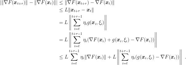
Therefore, using the triangle inequality, 


To rule out the case that 


Hi bremen79,
I want to cite your work, especially Lemma 1 and Theorem 2. Do you have some published paper about Theorem 2 so that I can include it as my reference?
Thank you!
LikeLike
Unfortunately, I didn’t publish it anywhere. I guess you can cite the blog post, I know of other people that are citing it 🙂
LikeLike
Hi, can you please give any reference to the equation “eta_t = min(1/L, \alpha/(\sigma*\sqrt(T))”? How to arrive at this equation?
LikeLike
In equation (1), first of all we need the left hand side to be big and positive. In particular, it is maximized for eta_t = 1/L and it is positive for any 0<= eta_t < =1/L, that gives the first condition in the min. With this condition the term eta_t-eta_t^2 L/2 is lower bounded by eta_t/2. So, now divide both terms by eta_t and on the right hand side we have (F(x_1)-F^*)/eta+sigma^2 L /2 T eta_t (because eta_t is constant). We want the right hand side to be as small as possible, so the best eta that minimizes this expression is eta_t=sqrt[(F(x_1)-F^*)/(sigma L T)]. Given that you don't know F(x_1)-F^*, you use some hyperparameter alpha that includes L too. This gives the second condition in the min. FYI, I didn't invent it, it is a standard reasoning for this kind of proofs.
LikeLike
Thanks for the great post!! Regarding Theorem 2, I am wondering how we know that we converge to a local minimum instead of a stationary point, since the gradient of the function in both cases is zero…
LikeLike
Good question! I think under reasonable assumptions it is possible to show that with probability 1 you end up in a local minimum, because saddle points are unstable equilibrium points for the algorithm. See for example this paper: http://proceedings.mlr.press/v49/lee16.pdf
LikeLike