Dynamic regret and ADER

In this post, we will see how to extend the notion of regret to a sequence of comparators instead of a single one. We saw that the definition of regret makes sense as a direct generalization of both the stochastic setting and the offline optimization. However, in some cases, we know that the environment is changing over time, so we would like an algorithm that guarantees a stronger notion of regret that captures the dynamics of the environment.

Our first extension is to use multiple comparators, using the concept of dynamic regret, defined as

$\displaystyle \text{D-Regret}({\boldsymbol u}_1, \dots, {\boldsymbol u}_T) :=\sum_{t=1}^T \ell_t({\boldsymbol x}_t) - \sum_{t=1}^T \ell_t({\boldsymbol u}_t),$

where ${{\boldsymbol u}_1, \dots, {\boldsymbol u}_T \in V}$ and ${V \subseteq {\mathbb R}^d}$ is the feasible set. For additional clarity, we will also refer to the standard notion of regret as the static regret.

Is it possible to obtain sublinear dynamic regret? We already know that in the case that ${{\boldsymbol u}_1= \dots= {\boldsymbol u}_T}$ it is possible because we recover the standard regret case. On the other hand, it should be intuitive that the problem becomes more and more difficult the more the sequence of ${{\boldsymbol u}_t}$ changes over time. There are various ways to quantity this complexity and a common one is the path-length ${P^{\phi}:V^T \rightarrow {\mathbb R}}$ defined as

$\displaystyle P^{\phi}({\boldsymbol u}_1, \dots, {\boldsymbol u}_T) :=\sum_{t=2}^T \phi({\boldsymbol u}_t-{\boldsymbol u}_{t-1}),$

where ${\phi:V\rightarrow {\mathbb R}}$ is a function that measures the shift from ${{\boldsymbol u}_{t-1}}$ to ${{\boldsymbol u}_t}$ . In particular, we will instantiate ${\phi}$ to be a norm. In the following, we will show how to design an online algorithm whose dynamic regret depends on the path length in the case that the feasible set is bounded.

1. Dynamic Regret of Online Mirror Descent

It turns out that some online learning algorithm already satisfies a dynamic regret without any additional change. For Online Mirror Descent (OMD), we can state the following theorem.

Theorem 1. Let ${B_\psi}$ the Bregman divergence w.r.t. ${\psi: X \rightarrow {\mathbb R}}$ and assume ${\psi}$ to be closed and ${\lambda}$ -strongly convex with respect to ${\|\cdot\|}$ in ${V\cap \mathop{\mathrm{int}} X}$ . Let ${V \subseteq X}$ a non-empty closed convex set. Assume that ${{\boldsymbol x}_t \in \mathop{\mathrm{int}} X}$ for ${t=1, \dots, T}$ . Then, ${\forall {\boldsymbol u}_1, \dots, {\boldsymbol u}_T \in V}$ , OMD with constant learning rate ${\eta}$ satisfies

$\displaystyle \text{D-Regret}({\boldsymbol u}_1, \dots, {\boldsymbol u}_T) \leq \frac{B_\psi({\boldsymbol u}_{T+1};{\boldsymbol x}_1) + Q P^{\|\cdot\|}({\boldsymbol u}_1, \dots, {\boldsymbol u}_T)}{\eta}+ \frac{\eta}{2\lambda} \sum_{t=1}^T \|{\boldsymbol g}_t\|^2_\star - \frac{B_\psi({\boldsymbol u}_{T+1}; {\boldsymbol x}_{T+1})}{\eta},$

where ${Q= \max_t \|\nabla \psi({\boldsymbol x}_t)-\nabla \psi({\boldsymbol x}_1)\|_\star}$ .

Proof: From the one-step inequality for OMD with competitor ${{\boldsymbol u}_t}$ , we have

$\displaystyle \begin{aligned} \eta(\ell_t({\boldsymbol x}_t)-\ell_t({\boldsymbol u}_t)) &\leq B_\psi({\boldsymbol u}_t;{\boldsymbol x}_t)-B_\psi({\boldsymbol u}_t;{\boldsymbol x}_{t+1}) + \frac{\eta^2}{2 \lambda} \|{\boldsymbol g}_t\|^2_\star\\ &=B_\psi({\boldsymbol u}_t;{\boldsymbol x}_t)-B_\psi({\boldsymbol u}_{t+1};{\boldsymbol x}_{t+1}) + B_\psi({\boldsymbol u}_{t+1};{\boldsymbol x}_{t+1}) - B_\psi({\boldsymbol u}_t;{\boldsymbol x}_{t+1}) + \frac{\eta_t^2}{2 \lambda} \|{\boldsymbol g}_t\|^2_\star~. \end{aligned}$

Dividing by ${\eta}$ and summing over time, we have

$\displaystyle \begin{aligned} \sum_{t=1}^T (\ell_t({\boldsymbol x}_t)-\ell_t({\boldsymbol u}_t)) &\leq \sum_{t=1}^T \frac{B_\psi({\boldsymbol u}_t;{\boldsymbol x}_t)-B_\psi({\boldsymbol u}_{t+1};{\boldsymbol x}_{t+1})}{\eta} + \sum_{t=1}^T \frac{B_\psi({\boldsymbol u}_{t+1};{\boldsymbol x}_{t+1}) - B_\psi({\boldsymbol u}_t;{\boldsymbol x}_{t+1})}{\eta} + \sum_{t=1}^T \frac{\eta}{2 \lambda} \|{\boldsymbol g}_t\|^2_\star \\ &= \frac{B_\psi({\boldsymbol u}_1;{\boldsymbol x}_1)-B_\psi({\boldsymbol u}_{T+1};{\boldsymbol x}_{T+1})}{\eta} + \sum_{t=1}^T \frac{B_\psi({\boldsymbol u}_{t+1};{\boldsymbol x}_{t+1}) - B_\psi({\boldsymbol u}_t;{\boldsymbol x}_{t+1})}{\eta} + \frac{\eta}{2\lambda} \sum_{t=1}^T \|{\boldsymbol g}_t\|^2_\star~. \end{aligned}$

Now observe that

$\displaystyle \begin{aligned} B_\psi&({\boldsymbol u}_{t+1};{\boldsymbol x}_{t+1}) - B_\psi({\boldsymbol u}_t;{\boldsymbol x}_{t+1})\\ &=\psi({\boldsymbol u}_{t+1})-\psi({\boldsymbol x}_{t+1})-\langle \nabla \psi({\boldsymbol x}_{t+1}), {\boldsymbol u}_{t+1}-{\boldsymbol x}_{t+1}) -\psi({\boldsymbol u}_t) +\psi({\boldsymbol x}_{t+1})+\langle \nabla \psi({\boldsymbol x}_{t+1}), {\boldsymbol u}_t-{\boldsymbol x}_{t+1}\rangle\\ &=\psi({\boldsymbol u}_{t+1})-\psi({\boldsymbol u}_t)+\langle \nabla \psi({\boldsymbol x}_1), {\boldsymbol u}_{t}-{\boldsymbol u}_{t+1}\rangle + \langle \nabla \psi({\boldsymbol x}_{t+1})-\nabla\psi({\boldsymbol x}_1), {\boldsymbol u}_{t}-{\boldsymbol u}_{t+1}\rangle~. \end{aligned}$

Hence, we have

$\displaystyle \begin{aligned} \sum_{t=1}^T &(B_\psi({\boldsymbol u}_{t+1};{\boldsymbol x}_{t+1}) - B_\psi({\boldsymbol u}_t;{\boldsymbol x}_{t+1}))\\ &=\psi({\boldsymbol u}_{T+1}) - \psi({\boldsymbol u}_1) + \langle \nabla \psi({\boldsymbol x}_1), {\boldsymbol u}_1-{\boldsymbol u}_{T+1}\rangle +\sum_{t=1}^T \langle \nabla \psi({\boldsymbol x}_{t+1})-\nabla\psi({\boldsymbol x}_1), {\boldsymbol u}_{t}-{\boldsymbol u}_{t+1}\rangle\\ &=B_\psi({\boldsymbol u}_{T+1}; {\boldsymbol x}_1)-B_\psi({\boldsymbol u}_1;{\boldsymbol x}_1)+\sum_{t=1}^T \langle \nabla \psi({\boldsymbol x}_{t+1})-\nabla\psi({\boldsymbol x}_1), {\boldsymbol u}_{t}-{\boldsymbol u}_{t+1}\rangle~. \end{aligned}$

Putting it all together, we have

$\displaystyle \begin{aligned} \text{D-Regret}({\boldsymbol u}_1, \dots, {\boldsymbol u}_T) &\leq \frac{B_\psi({\boldsymbol u}_{T+1};{\boldsymbol x}_1) - B_\psi({\boldsymbol u}_{T+1}; {\boldsymbol x}_{T+1})}{\eta}+ \frac{\eta}{2\lambda} \sum_{t=1}^T \|{\boldsymbol g}_t\|^2_\star\\ &\quad +\frac{1}{\eta}\sum_{t=1}^T \langle \nabla \psi({\boldsymbol x}_{t+1})-\nabla\psi({\boldsymbol x}_1), {\boldsymbol u}_{t}-{\boldsymbol u}_{t+1}\rangle~. \end{aligned}$

Assuming that ${\|\nabla \psi({\boldsymbol x}_t)-\nabla \psi({\boldsymbol x}_1)\|_\star \leq Q}$ and using the definition of dual norm, we have the stated bound. $\Box$

Assuming ${\|{\boldsymbol g}_t\|_\star \leq L}$ and selecting the usual learning rate ${\eta=\frac{\alpha \sqrt{2\lambda}}{L\sqrt{T}}}$ , we have

$\displaystyle \text{D-Regret}({\boldsymbol u}_1, \dots, {\boldsymbol u}_T) \leq \frac{\sqrt{2} L}{\sqrt{\lambda}} \left(\frac{B_\psi({\boldsymbol u}_{T+1};{\boldsymbol x}_1) + Q P^{\|\cdot\|}({\boldsymbol u}_1, \dots, {\boldsymbol u}_T)}{\alpha} + \alpha \right) \sqrt{T}~.$

In other words, we suffer an additional regret of

$\displaystyle \sqrt{2} L \frac{Q P^{\|\cdot\|}({\boldsymbol u}_1, \dots, {\boldsymbol u}_T)}{\alpha \sqrt{\lambda}} \sqrt{T}$

compared to the static case, for any ${{\boldsymbol u}_1, \dots, {\boldsymbol u}_T \in V}$ .

Example 1. Consider the case that the feasible is has diameter ${D}$ with respect to the L2 norm, i.e., ${D=\max_{{\boldsymbol x},{\boldsymbol y} \in V} \|{\boldsymbol x}-{\boldsymbol y}\|_2}$ . Set ${\psi({\boldsymbol x})=\frac12 \|{\boldsymbol x}\|_2^2}$ and assume the subgradients to satisfy ${\|{\boldsymbol g}_t\|_\star\leq L}$ for ${t=1, \dots, T}$ . In this case, we have that ${Q=D}$ and setting ${\eta=\frac{\alpha}{L \sqrt{T}}}$ we have

$\displaystyle \text{D-Regret}({\boldsymbol u}_1, \dots, {\boldsymbol u}_T) \leq \frac12 \left(\frac{D^2 + 2D \, P^{\|\cdot\|}({\boldsymbol u}_1, \dots, {\boldsymbol u}_T)}{\alpha} + \alpha\right) L \sqrt{T}~.$

Could we obtain a better regret guarantee? We could set the learning rate to ${\eta=\frac{\sqrt{2\lambda}\sqrt{B_\psi({\boldsymbol u}_{T+1};{\boldsymbol x}_1) + Q P^{\|\cdot\|}({\boldsymbol u}_1, \dots, {\boldsymbol u}_T)}}{L\sqrt{T}}}$ to obtain the dynamic regret

$\displaystyle \text{D-Regret}({\boldsymbol u}_1, \dots, {\boldsymbol u}_T) \leq \frac{\sqrt{2}}{\sqrt{\lambda}} L \sqrt{(B_\psi({\boldsymbol u}_{T+1};{\boldsymbol x}_1) + Q P^{\|\cdot\|}({\boldsymbol u}_1, \dots, {\boldsymbol u}_T))} \sqrt{T}~.$

However, assuming the knowledge of the exact value of ${P^{\|\cdot\|}}$ is an unreasonable assumption because it violates the assumption of the adversarial nature of the problem. This mirrors the problem of tuning the learning rate with the knowledge of ${\|{\boldsymbol x}_1-{\boldsymbol u}\|}$ in online gradient descent. Fortunately, there is a solution and we will see it in the next section.

2. ADER: Optimal Dependency on the Path Length for Online Subgradient Descent

In the previous section, we saw that the algorithm needs to know the path length of the competitors to tune its learning rate. Here, we show how to construct an online learning algorithm that achieves the same guarantees up to polylogarithmic terms. For simplicity, we will consider the Euclidean case, but it is easy to extend it to the Bregman case. Moreover, we assume the losses to be ${L}$ -Lipschitz w.r.t. the L2 norm.

We will use a classic online learning method: to run in parallel many projected Online Gradient Descent (OGD) algorithms with different learning rates and use an Exponentiated Gradient algorithm (EG) to learn online the best combination of their iterates. In this way, we will show that the cumulative loss of the resulting algorithm is close to the cumulative loss of the best learning rate, which in turn will give us the right dependency on the path length.

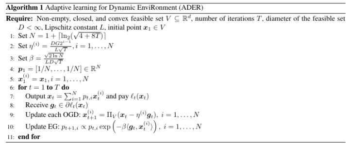
Consider a feasible set ${V}$ with bounded L2 diameter ${D}$ and assume of the losses ${\ell_t}$ to be ${L}$ -Lipschitz. Using projected OGD with learning rate ${\eta}$ , we obtain the following regret upper bound

$\displaystyle \text{D-Regret}({\boldsymbol u}_1, \dots, {\boldsymbol u}_T) \leq \frac12 \left(\frac{D^2 + 2D \, P^{\|\cdot\|_2}({\boldsymbol u}_1, \dots, {\boldsymbol u}_T)}{\eta} + \eta L^2\right) \sqrt{T}, \ \forall {\boldsymbol u}_1, \dots, {\boldsymbol u}_T\in V~.$

Using the fact that ${P^{\|\cdot\|_2}({\boldsymbol u}_1, \dots, {\boldsymbol u}_T)\leq D T}$ , the optimal choice of ${\eta^\star=\frac{\sqrt{D^2 + 2D \, P^{\|\cdot\|_2}({\boldsymbol u}_1, \dots, {\boldsymbol u}_T)}}{L \sqrt{T}}}$ satisfies

$\displaystyle \frac{D}{L\sqrt{T}} \leq \eta^\star \leq \frac{D\sqrt{1+2T}}{L\sqrt{T}}~.$

So, consider a grid of ${N=1+\lceil\ln_2 \sqrt{4+8T}\rceil}$ learning rates ${\eta^{(i)}=\frac{D 2^{i-1}}{L\sqrt{T}}, i=1, \dots, N}$ , so that ${\eta^{(1)}=\frac{D}{L\sqrt{T}}}$ and ${\eta^{(N)}\geq 2\frac{D\sqrt{1+2T}}{L\sqrt{T}}}$ . This implies that there exists ${i^\star}$ such that

$\displaystyle \eta^{(i^\star)} \leq \eta^\star \leq 2\eta^{(i^\star)}~.$

To combine the OGD algorithms with different learning rates, we use the EG algorithm where the OGD algorithms are our experts. We construct the loss vector for EG as ${{\boldsymbol z}_t = [\ell_t({\boldsymbol x}^{(1)}_{t}), \dots, \ell_t({\boldsymbol x}^{(N)}_{t})]^\top}$ . The EG algorithm is invariant to additive constants to the coordinates of the loss vector, hence we can consider it as if it were running on the losses ${\ell_t({\boldsymbol x}^{(i)})-\ell_t({\boldsymbol x}_1)}$ that makes them bounded in absolute value by ${D L}$ . Hence, using a uniform prior and learning rate ${\beta=\frac{\sqrt{2\ln N}}{L D \sqrt{T}}}$ , we obtain the regret

$\displaystyle \sum_{t=1}^T \langle {\boldsymbol p}_t, {\boldsymbol z}_t\rangle - \min_i \sum_{t=1}^T z_{t,i} \leq \sqrt{2} L\,D \sqrt{T \ln N}~.$

Now observe that by Jensen’s inequality and the convexity of ${\ell_t}$ , we have

$\displaystyle \langle {\boldsymbol p}_t, {\boldsymbol z}_t\rangle = \sum_{i=1}^N p_{t,i} \ell_t({\boldsymbol x}^{(i)}_t) \geq \ell_t\left(\sum_{i=1}^N p_{t,i} {\boldsymbol x}^{(i)}_t\right) = \ell_t({\boldsymbol x}_t)~.$

This motivates the choice of using a convex combination of the predictions of the OGD algorithms. Moreover, we have ${\min_i \sum_{t=1}^T z_{t,i}=\min_i \sum_{t=1}^T \ell_t({\boldsymbol x}^{(i)}_t)}$ . From the regret of OGD and the choice of ${\eta^{(i)}}$ , we have

$\displaystyle \min_i \sum_{t=1}^T \ell_t({\boldsymbol x}^{(i)}_t) \leq \sum_{t=1}^T \ell_t({\boldsymbol x}^{(i^\star)}_t) \leq \sum_{t=1}^T \ell_t({\boldsymbol u}_t) + \frac{3}{2} L \sqrt{T (D^2 + 2D \, P^{\|\cdot\|_2}({\boldsymbol u}_1, \dots, {\boldsymbol u}_T))} ,\ \forall {\boldsymbol u}_1, \dots, {\boldsymbol u}_T\in V~.$

Putting it all together, we have

$\displaystyle \begin{aligned} &\text{D-Regret}({\boldsymbol u}_1,\dots, {\boldsymbol u}_T)\\ &\quad = \sum_{t=1}^T (\ell_t({\boldsymbol x}_t)-\ell_t({\boldsymbol u}_t))\\ &\quad \leq \frac32 L \sqrt{T (D^2 + 2D \, P^{\|\cdot\|_2}({\boldsymbol u}_1, \dots, {\boldsymbol u}_T))} + \sqrt{2} L D \sqrt{T \ln \left(2+\ln_2 \sqrt{4+8T}\right)}, \ \forall {\boldsymbol u}_1, \dots, {\boldsymbol u}_T~. \end{aligned}$

We are still not completely done: This construction above queries ${N = O(\ln T)}$ subgradients in each step, so now we show how to reduce it to only one subgradient per iteration. This is easily achieved: It is enough to run the construction on the convex surrogate losses ${\tilde{\ell}_t({\boldsymbol x})=\langle {\boldsymbol g}_t, {\boldsymbol x}\rangle}$ , where ${{\boldsymbol g}_t\in \partial \ell_t({\boldsymbol x}_t)}$ . The advantage is that ${\partial \tilde{\ell}_t({\boldsymbol x}) = \{{\boldsymbol g}_t\}}$ for all ${{\boldsymbol x}}$ , hence all the OGD algorithms receive the same subgradient! Once again, we have that ${|\tilde{\ell}_t({\boldsymbol x}_t)-\tilde{\ell}_t({\boldsymbol x}_1)|\leq L \, D}$ . Moreover, we have

$\displaystyle \ell_t({\boldsymbol x}_t)-\ell_t({\boldsymbol u}_t) \leq \langle {\boldsymbol g}_t, {\boldsymbol x}_t-{\boldsymbol u}_t\rangle = \tilde{\ell}_t({\boldsymbol x}_t)-\tilde{\ell}_t({\boldsymbol u}_t), \ \forall {\boldsymbol u}_t \in V~.$

Hence, a dynamic regret guarantee on ${\tilde{\ell}_t}$ immediately translates to a dynamic regret guarantee on ${\ell_t}$ . The resulting algorithm is called Adaptive learning for Dynamic EnviRonment (ADER) and it is in Algorithm 1. Formally, we have the following theorem.

Theorem 2. Let ${V\subseteq {\mathbb R}^d}$ be a non-empty closed convex set with bounded diameter with respect to the L2 norm equal to ${D}$ . Assume ${\ell_t:V \rightarrow {\mathbb R}}$ to be convex functions subdifferentiable in ${V}$ and ${L}$ -Lipschitz with respect to the L2 norm. Then, ${\forall {\boldsymbol u}_1, \dots, {\boldsymbol u}_T \in V}$ , Algorithm 1 satisfies

$\displaystyle \begin{aligned} \text{D-Regret}({\boldsymbol u}_1,\dots, {\boldsymbol u}_T) \leq \frac32 L \sqrt{T(D^2 + 2D \, P^{\|\cdot\|_2}({\boldsymbol u}_1, \dots, {\boldsymbol u}_T))} + \sqrt{2} L D \sqrt{T \ln \left(2+\ln_2 \sqrt{4+8T}\right)}~. \end{aligned}$

Note that while we query only one subgradient per round, the computational complexity of ADER per round is still ${O(\ln T)}$ when ${T}$ goes to infinity. This is because in each round we need to update ${O(\ln T)}$ different OGD algorithms.

3. History Bits

Herbster&Warmuth (1998) introduced the idea of tracking the best expert in learning with experts game. In this setting, the best expert is allowed to change at most ${k}$ times. Zinkevich (2003) is often erroneously thought to have introduced the dynamic regret, while it first appeared in Herbster&Warmuth (1998), Herbster&Warmuth (2001), with upper bounds that depend on the drift ${\sum_{t=2}^T \|{\boldsymbol u}_t-{\boldsymbol u}_{t-1}\|_p}$ .

Theorem 1 is a generalization of Cesa-Bianchi&Lugosi (2006, Theorem 11.4) to arbitrary distance generating functions and considering Lipschitz losses. Also, following Jacobsen&Cutkosky (2022, Lemma 4), I have fixed the offset in the proof so that we do not have to assume that ${\boldsymbol{0} \in V}$ .

Zhang et al. (2018) designed the ADER algorithm and they also proved that it is optimal in bounded domains. The idea of combining online algorithms with different learning rates comes directly from the MetaGrad algorithm (van Erven&Koolen, 2016, van Erven et al., 2021) which also showed how to query a single gradient per round. In turn, MetaGrad is based on prior work using a grid of learning rates in EG (Koolen et al., 2014). By now, this is a well-known method that allows us to solve essentially all problems of tuning learning rates in bounded domains, at least theoretically. One can also combine different learning rates in unbounded domains, with a multi-scale expert algorithm (Foster et al., 2017, Cutkosky&Orabona, 2018). This method can be considered a better “doubling trick” because it allows tracking non-monotonic quantities at the price of a logarithmic computational overhead. It is worth also stressing that the general idea of combining the outputs of different online learning algorithms through another online learning algorithm is instead much older, and it goes back at least to Blum&Mansour (2005), Blum&Mansour (2007).

I described a slightly simpler version of ADER with a flat prior, see Exercise 1 for the original bound. I also removed the unnecessary assumption that ${\boldsymbol{0} \in V}$ . Recently, Zhao et al. (2020), Zhao et al. (2024) improved the guarantees of ADER using optimistic algorithms, obtaining smaller bounds in easy environments.

Acknowledgements

Thanks to Nicolò Campolongo for telling me about the papers by Blum and Mansour.

4. Exercises

Exercise 1. Change the prior in the EG algorithm to obtain a dependency of ${\ln \ln (1+P^{\|\cdot\|_2}({\boldsymbol u}_1, \dots, {\boldsymbol u}_T))}$ instead of ${\ln \ln T}$ . In this way, if the path length is zero, that is we are in the static case, the regret is ${O(\sqrt{T})}$ instead of ${O(\sqrt{T \ln \ln T})}$ , when ${T\rightarrow \infty}$ .