Better Optimistic Bounds and Delays as Bad Hints

We now consider online learning with delayed feedback. We consider a constant delay of length ${\tau}$ , where at time ${t}$ the learner has only observed ${\ell_1, \dots, \ell_{t-1-\tau}}$ before producing ${{\boldsymbol x}_t}$ . In other words, the learner observes ${\ell_t}$ at time ${t+\tau}$ . This means that the algorithm receives its first feedback at round ${\tau+1}$ and it receives no feedback before that round. We can expect that the delay will increase the regret of the algorithm and one can show that the optimal regret should depend on ${\tau}$ as ${\sqrt{\tau}}$ (Weinberger&Ordentlich, 2002). Let’s see how to achieve this optimal dependency.

1. Delay as Bad Hints

Instead of designing online algorithms specifically for the case of delayed feedback, we will reduce the setting of online learning with delays to the one of optimistic online learning, that is, when we receive the hint ${\tilde{{\boldsymbol g}}_t}$ at each round ${t}$ and we use it in optimistic algorithms. In particular, using FTRL with linearized losses with delays means that we predict with ${{\boldsymbol x}_t=\mathop{\mathrm{argmin}}_{{\boldsymbol x} \in \mathcal{V}} \ \psi_t({\boldsymbol x})}$ for ${t\leq \tau+1}$ and

$\displaystyle {\boldsymbol x}_t = \mathop{\mathrm{argmin}}_{{\boldsymbol x} \in \mathcal{V}} \ \psi_t({\boldsymbol x}) + \sum_{i=1}^{t-1-\tau} \langle {\boldsymbol g}_i, {\boldsymbol x}\rangle, \quad t \geq \tau+2~.$

On the other hand, in Optimistic FTRL without delays and linearized losses we predict with

$\displaystyle {\boldsymbol x}_t = \mathop{\mathrm{argmin}}_{{\boldsymbol x} \in \mathcal{V}} \ \psi_t({\boldsymbol x}) + \langle \tilde{{\boldsymbol g}}_t,{\boldsymbol x}\rangle +\sum_{i=1}^{t-1} \langle {\boldsymbol g}_i, {\boldsymbol x}\rangle~.$

Hence, the two updates are equivalent if we set ${\tilde{{\boldsymbol g}}_t= - \sum_{i=\max(1,t-\tau)}^{t-1} {\boldsymbol g}_i}$ . In other words, we are receiving a very bad hint that corresponds to the delayed feedback.

In the same way, we have that in OMD with delays we predict the same ${{\boldsymbol x}_1}$ for the first ${\tau+1}$ rounds and

$\displaystyle {\boldsymbol x}_{t+1} = \mathop{\mathrm{argmin}}_{{\boldsymbol x} \in \mathcal{V}} \ B_\psi({\boldsymbol x};{\boldsymbol x}_t) + \eta_{t} \langle {\boldsymbol g}_{t-\tau}, {\boldsymbol x}\rangle, \quad \forall t\geq \tau+1~.$

On the other hand, Optimistic OMD without delays updates with

$\displaystyle {\boldsymbol x}_{t+1} = \mathop{\mathrm{argmin}}_{{\boldsymbol x} \in \mathcal{V}} \ B_\psi({\boldsymbol x};{\boldsymbol x}_t) + \eta_{t} \langle {\boldsymbol g}_{t}+\tilde{{\boldsymbol g}}_{t+1}-\tilde{{\boldsymbol g}}_{t}, {\boldsymbol x}\rangle,$

where ${\tilde{{\boldsymbol g}}_1=\boldsymbol{0}}$ . So, the two are equivalent by setting ${\tilde{{\boldsymbol g}}_{t+1}-\tilde{{\boldsymbol g}}_{t}={\boldsymbol g}_{t-\tau}-{\boldsymbol g}_t}$ . So, unrolling, we have ${\tilde{{\boldsymbol g}}_{t+1}=-\sum_{i=\max(1,t-\tau+1)}^{t} {\boldsymbol g}_i}$ .

The above observations are very powerful because they can immediately give us the regret guarantee of FTRL and OMD with delays. Indeed, considering FTRL, assuming that the regularizer ${\psi_t({\boldsymbol x})}$ is ${\lambda_t}$ -strongly convex with respect to ${\|\cdot\|}$ , we have

$\displaystyle \sum_{t=1}^T \langle {\boldsymbol g}_t, {\boldsymbol x}_t-{\boldsymbol u}\rangle \leq \psi_{T+1}({\boldsymbol u}) - \min_{{\boldsymbol x} \in \mathcal{V}} \ \psi_1({\boldsymbol x}) + \sum_{t=1}^T \frac{\|\sum_{i=\max(1,t-\tau)}^{t} {\boldsymbol g}_i\|^2_\star}{2\lambda_t}, \quad \forall {\boldsymbol u} \in \mathcal{V}~.$

The result for OMD with delays is similar. The optimal tuning of ${\lambda_t}$ would give us a ${\mathcal{O}(\sqrt{T})}$ regret upper bound, but a linear dependency on ${\tau}$ . Unfortunately, according to what we said above, this is suboptimal…

Where is the problem? Is the reduction from delays to optimistic updates suboptimal? This seems unlikely, given that the reduction is exact. Instead, the problem is somewhere else: The optimistic bounds we have are suboptimal!

So, in the next two sections, we show a better bound for Optimistic OMD and Optimistic FTRL, which will imply the optimal bound for OMD and FTRL with delays.

2. Improved Optimistic OMD Bound

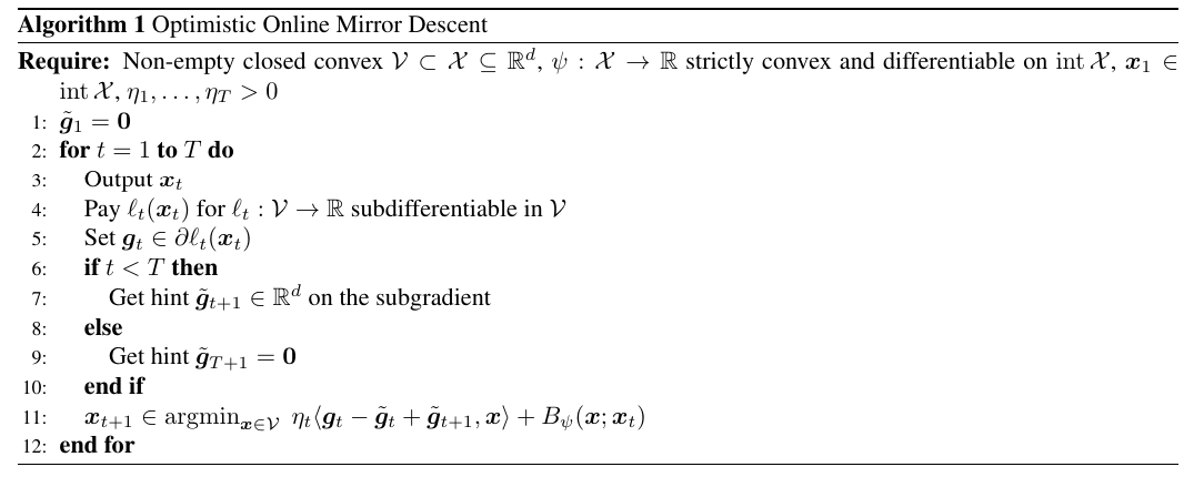
As we already saw, the following one is the pseudo-code of Optimistic OMD.

Note that setting ${\tilde{{\boldsymbol g}}_1=\boldsymbol{0}}$ is not a limitation because setting it to any other value would be equivalent to changing the arbitrary initial point ${{\boldsymbol x}_1}$ . In the same way, setting ${\tilde{{\boldsymbol g}}_{T+1}=\boldsymbol{0}}$ does not change in any way the behaviour of the algorithm in round ${t=1, \dots, T}$ , but it is needed to simplify the analysis.

We can now state its improved regret guarantee.

Theorem 1. Let ${B_\psi}$ be the Bregman divergence with respect to ${\psi: \mathcal{X} \rightarrow {\mathbb R}}$ and assume ${\psi}$ to be proper, closed, and ${\lambda}$ -strongly convex with respect to ${\|\cdot\|}$ in ${\mathcal{V}}$ . Let ${\mathcal{V} \subseteq \mathcal{X}}$ be a non-empty closed convex set. With the notation in Algorithm 1, assume each ${{\boldsymbol x}_{t+1}}$ exists and lies in ${\mathop{\mathrm{int}} \mathcal{X}}$ . Assume ${\eta_{t+1}\leq \eta_{t}}$ for ${t=1, \dots, T-1}$ . Define ${\delta_t=\max(\|{\boldsymbol g}_t-\tilde{{\boldsymbol g}}_t\|_\star-\|{\boldsymbol g}_t-\tilde{{\boldsymbol g}}_t+\tilde{{\boldsymbol g}}_{t+1}\|_\star,0)}$ . Then, ${\forall {\boldsymbol u} \in \mathcal{V}}$ , the following regret bounds hold

$\displaystyle \begin{aligned} \sum_{t=1}^T (\ell_t({\boldsymbol x}_t)- \ell_t({\boldsymbol u})) &\leq \frac{ \max_{1\leq t \leq T} \ B_\psi({\boldsymbol u};{\boldsymbol x}_t)}{\eta_{T}} + \sum_{t=1}^T \left(\langle {\boldsymbol g}_t-\tilde{{\boldsymbol g}}_t,{\boldsymbol x}_{t}-{\boldsymbol x}_{t+1}\rangle- \frac{1}{\eta_t} B_\psi({\boldsymbol x}_{t+1};{\boldsymbol x}_t)\right) \\ &\leq \frac{ \max_{1\leq t \leq T} \ B_\psi({\boldsymbol u};{\boldsymbol x}_t)}{\eta_{T}} + \frac{1}{2\lambda}\sum_{t=1}^T \eta_t (\|{\boldsymbol g}_t-\tilde{{\boldsymbol g}}_t\|^2_\star-\delta^2_t)\\ &\leq \frac{ \max_{1\leq t \leq T} \ B_\psi({\boldsymbol u};{\boldsymbol x}_t)}{\eta_{T}} + \frac{1}{2\lambda}\sum_{t=1}^T \eta_t \|{\boldsymbol g}_t-\tilde{{\boldsymbol g}}_t\|_\star\min(\|{\boldsymbol g}_t-\tilde{{\boldsymbol g}}_t\|_\star, 2 \|{\boldsymbol g}_t-\tilde{{\boldsymbol g}}_t+\tilde{{\boldsymbol g}}_{t+1}\|_\star)~. \end{aligned}$

Moreover, if ${\eta_t}$ is constant, i.e., ${\eta_t=\eta \ \forall t=1,\dots,T}$ , we have

$\displaystyle \begin{aligned} \sum_{t=1}^T (\ell_t({\boldsymbol x}_t)- \ell_t({\boldsymbol u})) &\leq \frac{B_\psi({\boldsymbol u};{\boldsymbol x}_1)}{\eta} + \sum_{t=1}^T \left(\langle {\boldsymbol g}_t-\tilde{{\boldsymbol g}}_t,{\boldsymbol x}_{t}-{\boldsymbol x}_{t+1}\rangle- \frac{1}{\eta} B_\psi({\boldsymbol x}_{t+1};{\boldsymbol x}_t)\right)\\ &\leq \frac{B_\psi({\boldsymbol u};{\boldsymbol x}_1)}{\eta} + \frac{\eta}{2\lambda}\sum_{t=1}^T (\|{\boldsymbol g}_t-\tilde{{\boldsymbol g}}_t\|^2_\star-\delta_t^2)\\ &\leq \frac{B_\psi({\boldsymbol u};{\boldsymbol x}_1)}{\eta} + \frac{\eta}{2\lambda}\sum_{t=1}^T \|{\boldsymbol g}_t-\tilde{{\boldsymbol g}}_t\|_\star\min(\|{\boldsymbol g}_t-\tilde{{\boldsymbol g}}_t\|_\star, 2 \|{\boldsymbol g}_t-\tilde{{\boldsymbol g}}_t+\tilde{{\boldsymbol g}}_{t+1}\|_\star)~. \end{aligned}$

To prove this improved theorem, we will use the following technical lemmas.

Lemma 2. Assume ${\psi:\mathcal{X}\rightarrow {\mathbb R}}$ to be ${\lambda}$ -strongly convex w.r.t. ${\|\cdot\|}$ and ${{\boldsymbol u} \in \mathop{\mathrm{int}} \mathcal{X}}$ . Let ${\mathcal{V}\subseteq \mathcal{X}}$ be convex. Let ${{\boldsymbol x}'=\mathop{\mathrm{argmin}}_{{\boldsymbol x} \in \mathcal{V}} \ B_\psi({\boldsymbol x};{\boldsymbol u}) + \eta\langle {\boldsymbol g},{\boldsymbol x}\rangle}$ . Then, we have

$\displaystyle \|{\boldsymbol x}'-{\boldsymbol u}\| \leq \frac{\eta}{\lambda} \|{\boldsymbol g}\|_\star~.$

Proof: Observe that from the optimality condition on ${{\boldsymbol x}'}$ , we have

$\displaystyle \label{eq:lemma:diff_iterate_omd_eq1} \langle \eta {\boldsymbol g}+\nabla \psi({\boldsymbol x}')-\nabla \psi({\boldsymbol u}), {\boldsymbol v}-{\boldsymbol x}'\rangle\geq 0, \quad \forall {\boldsymbol v} \in \mathcal{V}~. \ \ \ \ \ (1)$

Hence, we have

$\displaystyle \lambda \|{\boldsymbol x}'-{\boldsymbol u}\|^2 \leq B_\psi({\boldsymbol u};{\boldsymbol x}')+B_\psi({\boldsymbol x}';{\boldsymbol u}) = \langle \nabla \psi({\boldsymbol x}') - \nabla \psi({\boldsymbol u}), {\boldsymbol x}'-{\boldsymbol u}\rangle \leq \langle \eta {\boldsymbol g}, {\boldsymbol x}' - {\boldsymbol u}\rangle \leq \eta \|{\boldsymbol g}\|_\star \|{\boldsymbol x}'-{\boldsymbol u}\|~.$

where in first inequality we used the strong convexity of ${\psi}$ , (1) in the second one, and the definition of dual norms in the last one. Reordering, we have the stated bound. $\Box$

Lemma 3. Let ${{\boldsymbol g} \in {\mathbb R}^d}$ and ${a,c>0}$ . Then, we have

$\displaystyle \sup_{{\boldsymbol v} \in {\mathbb R}^d: \|{\boldsymbol v}\|\leq c/a} \ \langle {\boldsymbol g},{\boldsymbol v}\rangle - \frac{a}{2}\|{\boldsymbol v}\|^2 = \frac{1}{2 a } \left[\|{\boldsymbol g}\|^2_\star-\max(\|{\boldsymbol g}\|_\star-c,0)^2\right] \leq \frac{1}{2 a } \|{\boldsymbol g}\|_\star \min\left(\|{\boldsymbol g}\|_\star, 2 c \right)~.$

Proof:

$\displaystyle \begin{aligned} \sup_{{\boldsymbol v} \in {\mathbb R}^d: \|{\boldsymbol v}\|\leq c/a} \ \langle {\boldsymbol g},{\boldsymbol v}\rangle - \frac{a}{2}\|{\boldsymbol v}\|^2 &=\sup_{0\leq x\leq c/a} \ \sup_{{\boldsymbol v} \in {\mathbb R}^d: \|{\boldsymbol v}\|= x} \ \langle {\boldsymbol g},{\boldsymbol v}\rangle - \frac{a}{2}\|{\boldsymbol v}\|^2\\ &=\sup_{0\leq x\leq c/a} \ x\|{\boldsymbol g}\|_\star - \frac{a}{2}x^2\\ &=\frac{1}{a} \min(\|{\boldsymbol g}\|_\star,c)\left[\|{\boldsymbol g}\|_\star-\frac{1}{2}\min(\|{\boldsymbol g}\|_\star,c)\right]\\ &=\frac{1}{2a} \left[\|{\boldsymbol g}\|^2_\star-\max(\|{\boldsymbol g}\|_\star-c,0)^2\right]~. \end{aligned}$

The second inequality is obtained by lower bounding the max with its two possible values and overapproximating. $\Box$

We can now prove the Theorem.

Proof: We can use the one-step lemma for OMD with ${{\boldsymbol g}_t \rightarrow {\boldsymbol g}_t - \tilde{{\boldsymbol g}}_t + \tilde{{\boldsymbol g}}_{t+1}}$ , to have

$\displaystyle \langle {\boldsymbol g}_t - \tilde{{\boldsymbol g}}_t + \tilde{{\boldsymbol g}}_{t+1}, {\boldsymbol x}_t - {\boldsymbol u}\rangle \leq \frac{1}{\eta_t}\left(B_\psi({\boldsymbol u};{\boldsymbol x}_t) - B_\psi({\boldsymbol u};{\boldsymbol x}_{t+1}) - B_\psi({\boldsymbol x}_{t+1};{\boldsymbol x}_t)\right) + \langle {\boldsymbol g}_t - \tilde{{\boldsymbol g}}_t + \tilde{{\boldsymbol g}}_{t+1}, {\boldsymbol x}_t - {\boldsymbol x}_{t+1} \rangle~.$

Summing over ${t=1,\dots,T}$ the l.h.s., we obtain

$\displaystyle \begin{aligned} \sum_{t=1}^T \langle {\boldsymbol g}_t - \tilde{{\boldsymbol g}}_t + \tilde{{\boldsymbol g}}_{t+1}, {\boldsymbol x}_t - {\boldsymbol u}\rangle &= \sum_{t=1}^T \langle {\boldsymbol g}_t, {\boldsymbol x}_t - {\boldsymbol u}\rangle + \sum_{t=1}^T \langle \tilde{{\boldsymbol g}}_{t+1} -\tilde{{\boldsymbol g}}_t, {\boldsymbol x}_t-{\boldsymbol u}\rangle \\ &= \sum_{t=1}^T \langle {\boldsymbol g}_t, {\boldsymbol x}_t - {\boldsymbol u}\rangle + \langle \tilde{{\boldsymbol g}}_{1} - \tilde{{\boldsymbol g}}_{T+1}, {\boldsymbol u}\rangle + \sum_{t=1}^T \langle \tilde{{\boldsymbol g}}_{t+1} - \tilde{{\boldsymbol g}}_t, {\boldsymbol x}_t\rangle~. \end{aligned}$

Summing the r.h.s., we have that

$\displaystyle \begin{aligned} \sum_{t=1}^T \langle {\boldsymbol g}_t - \tilde{{\boldsymbol g}}_t + \tilde{{\boldsymbol g}}_{t+1}, {\boldsymbol x}_t - {\boldsymbol x}_{t+1} \rangle &= \sum_{t=1}^T \langle {\boldsymbol g}_t-\tilde{{\boldsymbol g}}_{t}, {\boldsymbol x}_t - {\boldsymbol x}_{t+1} \rangle + \sum_{t=1}^T \langle \tilde{{\boldsymbol g}}_{t+1}, {\boldsymbol x}_t - {\boldsymbol x}_{t+1} \rangle~. \end{aligned}$

Finally, observe that

$\displaystyle \sum_{t=1}^T \langle \tilde{{\boldsymbol g}}_{t+1} - \tilde{{\boldsymbol g}}_t, {\boldsymbol x}_t\rangle - \sum_{t=1}^T \langle \tilde{{\boldsymbol g}}_{t+1}, {\boldsymbol x}_t - {\boldsymbol x}_{t+1} \rangle = \sum_{t=1}^T (\langle \tilde{{\boldsymbol g}}_{t+1},{\boldsymbol x}_{t+1}\rangle -\langle \tilde{{\boldsymbol g}}_t,{\boldsymbol x}_t\rangle) = \langle \tilde{{\boldsymbol g}}_{T+1},{\boldsymbol x}_{T+1}\rangle - \langle \tilde{{\boldsymbol g}}_1,{\boldsymbol x}_1\rangle~.$

Telescoping the terms with the Bregman divergences gives the first bound.

Now, using the strong convexity of ${\psi}$ , we have

$\displaystyle \langle {\boldsymbol g}_t-\tilde{{\boldsymbol g}}_t,{\boldsymbol x}_{t}-{\boldsymbol x}_{t+1}\rangle- \frac{1}{\eta_t} B_\psi({\boldsymbol x}_{t+1};{\boldsymbol x}_t) \leq \langle {\boldsymbol g}_t-\tilde{{\boldsymbol g}}_t,{\boldsymbol x}_{t}-{\boldsymbol x}_{t+1}\rangle- \frac{\lambda}{2 \eta_t} \|{\boldsymbol x}_t-{\boldsymbol x}_{t+1}\|^2~.$

From Lemma 2, we know that ${\|{\boldsymbol x}_{t}-{\boldsymbol x}_{t+1}\|}$ is upper bounded by ${\frac{\eta_t}{\lambda}\|{\boldsymbol g}_t-\tilde{{\boldsymbol g}}_t+\tilde{{\boldsymbol g}}_{t+1}\|_\star}$ . Hence, we have

$\displaystyle \langle {\boldsymbol g}_t-\tilde{{\boldsymbol g}}_t,{\boldsymbol x}_{t}-{\boldsymbol x}_{t+1}\rangle- \frac{\lambda}{2 \eta_t} \|{\boldsymbol x}_t-{\boldsymbol x}_{t+1}\|^2 \leq \max_{{\boldsymbol v}\in {\mathbb R}^d: \|{\boldsymbol v}\|\leq \frac{\eta_t}{\lambda}\|{\boldsymbol g}_t-\tilde{{\boldsymbol g}}_t+\tilde{{\boldsymbol g}}_{t+1}\|_\star} \ \langle {\boldsymbol g}_t-\tilde{{\boldsymbol g}}_t,{\boldsymbol v}\rangle- \frac{\lambda}{2 \eta_t} \|{\boldsymbol v}\|^2~.$

Using Lemma 3 gives the second bound.

The bound for fixed ${\eta}$ is proved in a similar way. $\Box$

The advantage of these bounds is that the terms in the sum only depends linearly on bad hints, rather than quadratically. Next, we will use exactly this property to obtain the optimal regret guarantee for OMD with delayed feedback.

From Optimistic OMD to Delayed OMD. We now show the improved bound for OMD with delays and constant learning rate. The delay-to-optimism conversion says that we have to set ${\tilde{{\boldsymbol g}}_{t+1}=-\sum_{i=\max(1,t-\tau+1)}^{t} {\boldsymbol g}_i}$ for ${t=1, \dots, T-1}$ , yet we must set ${\tilde{{\boldsymbol g}}_{T+1}=\boldsymbol{0}}$ for the Optimistic OMD proof. Hence, we obtain a reduced term in the sum for the first ${T-1}$ rounds:

$\displaystyle \label{eq:delayed_omd} \sum_{t=1}^T \langle {\boldsymbol g}_t, {\boldsymbol x}_t-{\boldsymbol u}\rangle \leq \frac{B_\psi({\boldsymbol u};{\boldsymbol x}_1)}{\eta} + \frac{\eta}{\lambda} \sum_{t=\tau+1}^{T-1} \left\|\sum_{i=\max(1,t-\tau)}^{t} {\boldsymbol g}_i\right\|_\star \|{\boldsymbol g}_{t-\tau}\|_\star + \frac{\eta}{2\lambda} \left\|\sum_{i=\max(1,T-\tau)}^{T} {\boldsymbol g}_i\right\|^2_\star, \quad \forall {\boldsymbol u} \in \mathcal{V}~. \ \ \ \ \ (2)$

That is, assuming ${{\boldsymbol g}_t}$ bounded for all ${t}$ , we improved the worst-case dependency in the dominant term of the bound from ${\tau^2}$ to ${\tau}$ . Choosing the learning rate in the optimal way, we obtain the optimal regret guarantee of ${\mathcal{O}(\sqrt{\tau T})}$ .

3. Improved Optimistic FTRL Bound for Linear Losses

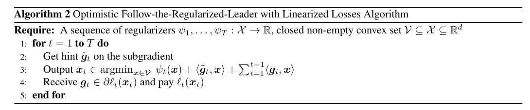
We now prove a similar improved regret guarantee for Optimistic FTRL with linearized losses, whose pseudo-code is the following one.

Here, we will give an improved version of the regret bound for Optimistic FTRL with linearized losses. The analysis will use an auxiliary sequence of predictions, and then relate these predictions to the ones of Optimistic FTRL.

Define ${{\boldsymbol x}^{(a)}_t}$ for ${t=1, \dots, T}$ the auxiliary sequence of predictions obtained with Optimistic FTRL with linearized losses with losses ${\ell_t({\boldsymbol x})=\langle {\boldsymbol g}_t, {\boldsymbol x}\rangle}$ and hints ${\tilde{{\boldsymbol g}}^{(a)}_t}$ . Given that this auxiliary sequence is only used in the analysis, we do not have to specify the choice of the hints ${\tilde{{\boldsymbol g}}^{(a)}_t}$ . Instead, we will leave them free, and state the final bound for any of these choices. Formally, defining ${F^{(a)}_t({\boldsymbol x}):=\psi_t({\boldsymbol x}) + \langle \tilde{{\boldsymbol g}}^{(a)}_t, {\boldsymbol x}\rangle + \sum_{i=1}^{t-1} \langle {\boldsymbol g}_i, {\boldsymbol x}\rangle}$ we have ${{\boldsymbol x}^{(a)}_t = \mathop{\mathrm{argmin}}_{{\boldsymbol x} \in \mathcal{V}} \ F^{(a)}_t({\boldsymbol x})}$ .

Theorem 4. With the notation in Algorithm 2, let ${\mathcal{V}}$ be convex, closed, non-empty. For ${t=1, \dots, T}$ , if ${\psi_t}$ is closed, subdifferentiable, and ${\lambda_t}$ -strongly convex with respect to ${\|\cdot\|}$ in ${\mathcal{V}}$ , then ${{\boldsymbol x}_t}$ exists and is unique. Moreover, if in addition ${\psi_{t+1}\geq \psi_t}$ pointwise for all ${t}$ , we have

$\displaystyle \begin{aligned} \sum_{t=1}^T &\ell_t({\boldsymbol x}_t) - \sum_{t=1}^T \ell_t({\boldsymbol u})\\ &\leq \sum_{t=1}^T \langle{\boldsymbol g}_t, {\boldsymbol x}_t - {\boldsymbol u}\rangle\\ &\leq \psi_{T+1}({\boldsymbol u}) - \min_{{\boldsymbol x} \in \mathcal{V}} \ \psi_{1}({\boldsymbol x}) + \sum_{t=1}^T \left[\frac{\|{\boldsymbol g}_t-\tilde{{\boldsymbol g}}^{(a)}_t\|_\star^2}{2\lambda_t} + \frac{\|{\boldsymbol g}_t\|_\star \|\tilde{{\boldsymbol g}}_t - \tilde{{\boldsymbol g}}^{(a)}_t\|_\star}{\lambda_t} \right], \end{aligned}$

for all ${{\boldsymbol u} \in \mathcal{V}}$ and all ${\tilde{{\boldsymbol g}}^{(a)}_t \in {\mathbb R}^d}$ for ${t=1, \dots, T}$ .

To prove this theorem we will need the following stability lemma for FTRL.

Lemma 5. Assume ${\psi:\mathcal{V} \rightarrow {\mathbb R}}$ to be ${\lambda}$ -strongly convex with respect to ${\|\cdot\|}$ . Define ${{\boldsymbol x}^{(1)} := \mathop{\mathrm{argmin}}_{{\boldsymbol x} \in \mathcal{V}} \ \psi({\boldsymbol x})+\langle {\boldsymbol \theta}^{(1)},{\boldsymbol x}\rangle}$ and ${{\boldsymbol x}^{(2)} := \mathop{\mathrm{argmin}}_{{\boldsymbol x} \in \mathcal{V}} \ \psi({\boldsymbol x})+\langle {\boldsymbol \theta}^{(2)},{\boldsymbol x}\rangle}$ . Then, ${\|{\boldsymbol x}^{(1)}-{\boldsymbol x}^{(2)}\|\leq \frac{1}{\lambda} \|{\boldsymbol \theta}^{(1)}-{\boldsymbol \theta}^{(2)}\|_\star}$ .

Proof: Define ${F^{(1)}:=\psi({\boldsymbol x})+\langle {\boldsymbol \theta}^{(1)},{\boldsymbol x}\rangle}$ and ${F^{(2)}=\psi({\boldsymbol x})+\langle {\boldsymbol \theta}^{(2)},{\boldsymbol x}\rangle}$ . From the strong convexity of ${\psi}$ , we have

$\displaystyle \begin{aligned} F^{(1)}({\boldsymbol x}^{(2)})-F^{(1)}({\boldsymbol x}^{(1)}) &\geq \frac{\lambda}{2}\|{\boldsymbol x}^{(1)}-{\boldsymbol x}^{(2)}\|^2\\ F^{(2)}({\boldsymbol x}^{(1)})-F^{(2)}({\boldsymbol x}^{(2)}) &\geq \frac{\lambda}{2}\|{\boldsymbol x}^{(1)}-{\boldsymbol x}^{(2)}\|^2~. \end{aligned}$

Hence, summing these two inequalities, we have

$\displaystyle \|{\boldsymbol \theta}^{(1)}-{\boldsymbol \theta}^{(2)}\|_\star \, \|{\boldsymbol x}^{(2)}-{\boldsymbol x}^{(1)}\| \geq \langle {\boldsymbol \theta}^{(1)}-{\boldsymbol \theta}^{(2)}, {\boldsymbol x}^{(2)}-{\boldsymbol x}^{(1)}\rangle \geq \lambda\|{\boldsymbol x}^{(1)}-{\boldsymbol x}^{(2)}\|^2,$

that completes the proof. $\Box$

We can now prove Theorem 4.

Proof: Using the regret bound for optimistic FTRL on the predictions ${{\boldsymbol x}^{(a)}_t}$ , we can now upper bound the regret of ${{\boldsymbol x}_t}$ as

$\displaystyle \begin{aligned} \sum_{t=1}^T \langle {\boldsymbol g}_t, {\boldsymbol x}_t-{\boldsymbol u}\rangle &= \sum_{t=1}^T \langle {\boldsymbol g}_t, {\boldsymbol x}^{(a)}_t-{\boldsymbol u}\rangle + \sum_{t=1}^T \langle {\boldsymbol g}_t, {\boldsymbol x}_t-{\boldsymbol x}^{(a)}_t\rangle\\ &\leq \psi_{T+1}({\boldsymbol u}) - \psi_1({\boldsymbol x}^{(a)}_1) + \sum_{t=1}^T \frac{\|{\boldsymbol g}_t -\tilde{{\boldsymbol g}}^{(a)}_t\|^2_\star}{2\lambda_t} + \sum_{t=1}^T \|{\boldsymbol g}_t\|_\star \|{\boldsymbol x}_t - {\boldsymbol x}^{(a)}_t\|\\ &\leq \psi_{T+1}({\boldsymbol u}) - \min_{{\boldsymbol x} \in \mathcal{V}} \ \psi_1({\boldsymbol x}) + \sum_{t=1}^T \frac{\|{\boldsymbol g}_t -\tilde{{\boldsymbol g}}^{(a)}_t\|^2_\star}{2\lambda_t} + \sum_{t=1}^T \|{\boldsymbol g}_t\|_\star \|{\boldsymbol x}_t - {\boldsymbol x}^{(a)}_t\| , \quad \forall {\boldsymbol u} \in \mathcal{V}~. \end{aligned}$

Now, we focus our attention on ${\|{\boldsymbol x}_t - {\boldsymbol x}^{(a)}_t\|}$ . From Lemma 5, we have ${\|{\boldsymbol x}_t^{(a)}-{\boldsymbol x}_t\|\leq \frac{1}{\lambda_t} \|\tilde{{\boldsymbol g}}_t-\tilde{{\boldsymbol g}}^{(a)}_t\|_\star}$ .

Using this inequality in the regret bound above, for any ${\tilde{{\boldsymbol g}}_1^{(a)}, \dots, \tilde{{\boldsymbol g}}^{(a)}_T}$ and any ${{\boldsymbol u} \in \mathcal{V}}$ , we have

$\displaystyle \begin{aligned} \sum_{t=1}^T \langle {\boldsymbol g}_t, {\boldsymbol x}_t-{\boldsymbol u}\rangle &= \sum_{t=1}^T \langle {\boldsymbol g}_t, {\boldsymbol x}^{(a)}_t-{\boldsymbol u}\rangle + \sum_{t=1}^T \langle {\boldsymbol g}_t, {\boldsymbol x}_t-{\boldsymbol x}^{(a)}_t\rangle\\ &\leq \psi_{T+1}({\boldsymbol u}) - \min_{{\boldsymbol x} \in \mathcal{V}} \ \psi_1({\boldsymbol x}) + \sum_{t=1}^T \left(\frac{\|{\boldsymbol g}_t -\tilde{{\boldsymbol g}}^{(a)}_t\|^2_\star}{2\lambda_t} + \frac{\|{\boldsymbol g}_t\|_\star \|\tilde{{\boldsymbol g}}_t - \tilde{{\boldsymbol g}}^{(a)}_t\|_\star}{\lambda_t}\right)~. \end{aligned}$

Remember that ${\tilde{{\boldsymbol g}}^{(a)}_t}$ is only used in the analysis. So, this upper bound holds for any choice of ${\tilde{{\boldsymbol g}}^{(a)}_t}$ . $\Box$

Note that the minimization with respect to ${\tilde{{\boldsymbol g}}_t^{(a)}}$ can be solved only with the knowledge of the dual norm used. However, we have the following upper bound (proof left as exercise, see Exercise 1)

$\displaystyle \min_{\tilde{{\boldsymbol g}}_t^{(a)}} \ \frac{\|{\boldsymbol g}_t -\tilde{{\boldsymbol g}}_t^{(a)}\|^2_\star}{2} +\|{\boldsymbol g}_t\|_\star \|\tilde{{\boldsymbol g}}_t - \tilde{{\boldsymbol g}}_t^{(a)}\|_\star \leq \frac{1}{2} \left[\|{\boldsymbol g}_t -\tilde{{\boldsymbol g}}_t\|^2_\star - \max(\|{\boldsymbol g}_t -\tilde{{\boldsymbol g}}_t\|_\star-\|{\boldsymbol g}_t\|_\star,0)^2\right]~.$

From Optimistic FTRL to Delayed FTRL. For our aim of analyzing online learning with delays, we can choose ${\tilde{{\boldsymbol g}}^{(a)}_t={\boldsymbol g}_t}$ . Then, using the obtained bound in the delay-to-optimism conversion, we have that FTRL with delayed linearized losses and increasing regularizer satisfies

$\displaystyle \label{eq:delayed_ftrl} \sum_{t=1}^T \langle {\boldsymbol g}_t, {\boldsymbol x}_t-{\boldsymbol u}\rangle \leq \psi_{T+1}({\boldsymbol u}) - \min_{{\boldsymbol x} \in \mathcal{V}} \ \psi_1({\boldsymbol x}) + \sum_{t=1}^T \frac{\|{\boldsymbol g}_t\|_\star \|\sum_{i=\max(1,t-\tau)}^{t} {\boldsymbol g}_i\|_\star}{\lambda_t}, \quad \forall {\boldsymbol u} \in \mathcal{V}~. \ \ \ \ \ (3)$

That is, assuming that the ${{\boldsymbol g}_t}$ are bounded, we improved the dependency in the sum from ${\mathcal{O}(\tau^2)}$ to ${\mathcal{O}(\tau)}$ . Choosing the strong convexity of the regularizer in the optimal way, we obtain the optimal regret guarantee of ${\mathcal{O}(\sqrt{\tau T})}$ .

4. Conclusion

I have described only the basic idea behind the reduction from online learning with delayed feedback to optimistic updates with bad hints. It should be immediate to see that this reduction allows us to use any variant for optimistic updates to study delayed updates. For example, it is now immediate to use data-depedent learning rates or regularizers to obtain tigher regret bounds under particular situations.

5. History Bits

Weinberger&Ordentlich (2002) were the first to analyze the delayed feedback problem. They considered the adversarial full information setting with a fixed, known delay ${\tau}$ . They achieved the optimal rate by proposing a black-box reduction, by running ${\tau+1}$ online algorithms on subsampled sequences. Zinkevich et al. (2009) analyzed OMD with delayed feedback and obtained the optimal regret. Joulani et al. (2013) unified most of the prior research on the effect of delay in adversarial and stochastic problems. McMahan&Streeter (2014) studied a variant of AdaGrad with delays. Quanrud&Khashabi (2015) studied OGD and FTRL with adversarially chosen delays, while Joulani et al. (2016) studied OMD and FTRL-Proximal with adaptive learning rates.

The equivalence of delays/bad hints and the improved regret guarantees for Optimistic FTRL and Optimistic OMD are due to Flaspohler et al. (2021). However, their OMD bound contains a small mistake: They are missing the last terms in the bound, due to the fact that we set the ${\tilde{{\boldsymbol g}}_{T+1}=\boldsymbol{0}}$ breaking the equivalence between optimistic and delayed updates for ${{\boldsymbol x}_{T+1}}$ . Note that while the choice of ${{\boldsymbol x}_{T+1}}$ does not influence the algorithm in the rounds ${1, \dots, T}$ , its value appears in the regret upper bound. (As soon as we have time, we will fix the arxiv version of Flaspohler et al. (2021)…) Flaspohler et al. (2021) also show that RM and RM+ automatically adapts to the delay ${\tau}$ .

Lemma 2 is from Joulani et al. (2016).

Acknowledgments

Thanks for ChatGPT 5.2 for checking the proofs. (Yet, I found the mistake in the previous paper, while ChatGPT 5.2 was claiming that everything was correct!)

6. Exercises

Exercise 1. Let ${{\boldsymbol g}, \tilde{{\boldsymbol g}} \in {\mathbb R}^d}$ and ${\|\cdot\|_\star}$ a norm. Then, show that

$\displaystyle \min_{\tilde{{\boldsymbol g}}^{(a)}} \ \frac{\|{\boldsymbol g} -\tilde{{\boldsymbol g}}^{(a)}\|^2_\star}{2} +\|{\boldsymbol g}\|_\star \|\tilde{{\boldsymbol g}} - \tilde{{\boldsymbol g}}^{(a)}\|_\star \leq \frac{1}{2} \left[\|{\boldsymbol g} -\tilde{{\boldsymbol g}}\|^2_\star - \max(\|{\boldsymbol g} -\tilde{{\boldsymbol g}}\|_\star-\|{\boldsymbol g}\|_\star,0)^2\right]~.$