From Online Learning to Non-convex Non-smooth Optimization

This is the last post in this series to show that online learning is more than online learning. This time it is about using an online linear optimization algorithm to minimize non-convex, non-smooth functions with access to stochastic gradients. Unlike in the previous two posts, here we will actually use the online algorithm itself, not just its regret guarantee. Nevertheless, the same philosophy applies: a regret guarantee is a statement that the sequence ${{\boldsymbol x}_1, \dots, {\boldsymbol x}_T}$ produced by the online algorithm has certain useful properties. So, even though the online linear optimization algorithm only minimizes linear functions, it can be used to design an optimization algorithm for non-convex functions.

1. From Online Learning to Non-Convex Non-Smooth Optimization

This section describes a simple (and surprisingly sharp) reduction from Online Linear Optimization (OLO) to the task of finding approximate stationary points of non-convex, non-smooth objectives. The key idea is to feed stochastic gradients to an online algorithm, which then decides the updates rather than the iterates.

We consider the objective function ${F:{\mathbb R}^d\rightarrow{\mathbb R}}$ , which is differentiable but not necessarily smooth, i.e., the gradient map might not be Lipschitz.

Example 1. Consider ${F:{\mathbb R} \rightarrow {\mathbb R}}$ defined as ${F(x)=\frac{2}{3}|x|^\frac{3}{2}}$ . Then, ${F'(x)=\rm sign(x) \sqrt{|x|}}$ , where ${\rm sign(0):=0}$ . Hence, ${F}$ is differentiable everywhere, but its derivative is not Lipschitz because ${F''(x)}$ is unbounded when ${x \rightarrow 0}$ .

To connect function values to gradients without convexity or smoothness, we isolate the only calculus identity needed by the reduction. So, we will define well-behaved functions as those that satisfy the specific equality we need.

Definition 1 (Well-behaved function). A differentiable function ${F:{\mathbb R}^d\rightarrow{\mathbb R}}$ is well-behaved if for every ${{\boldsymbol x},{\boldsymbol y}\in{\mathbb R}^d}$ ,

$\displaystyle \label{eq:well-behaved} F({\boldsymbol y})-F({\boldsymbol x}) = \int_0^1 \! \langle \nabla F({\boldsymbol x}+t({\boldsymbol y}-{\boldsymbol x})), {\boldsymbol y}-{\boldsymbol x}\rangle \, \mathrm{d} t~. \ \ \ \ \ (1)$

Remark 1. Identity (1) is immediate for smooth functions (by the fundamental theorem of calculus applied to ${t\mapsto F({\boldsymbol x}+t({\boldsymbol y}-{\boldsymbol x}))}$ ), but it can hold well beyond smooth objectives. In particular, Cutkosky et al. (2023) show that if ${F}$ is locally Lipschitz then an arbitrarily small randomized smoothing yields a differentiable well-behaved surrogate with a natural stochastic gradient oracle. Here, we focus on the differentiable well-behaved case to keep the presentation simple.

We now define our notion of optimality. Since ${F}$ is non-convex and not necessarily smooth, small gradients are not obviously implied by function decrease; we instead certify a local averaged stationarity notion that measures how close we are to a local minimum by considering local averages of gradients.

Definition 2 (Barycentric ${(\delta,\epsilon)}$ -stationarity). Let ${F}$ be differentiable almost everywhere, and let ${\delta>0}$ . Let ${\mathcal{Q}({\boldsymbol x},\delta)}$ be the set of random variables ${{\boldsymbol Q}}$ with finite support in the ball of radius ${\delta}$ around ${{\boldsymbol x}}$ , such that ${\nabla F({\boldsymbol y})}$ exists for all ${{\boldsymbol y}}$ in the support of ${{\boldsymbol Q}}$ . Define

$\displaystyle \|\nabla F({\boldsymbol x})\|_\delta \stackrel{\text{def}}{=} \inf_{{\boldsymbol Q} \in \mathcal{Q}({\boldsymbol x},\delta)} \ \left\{ \left\| \mathop{\mathbb E}\left[\nabla F({\boldsymbol Q})\right]\right\|_2 : \mathop{\mathbb E}[{\boldsymbol Q}]={\boldsymbol x} \right\}~.$

We say that ${{\boldsymbol x}}$ is a barycentric ${(\delta,\epsilon)}$ -stationary point if ${\|\nabla F({\boldsymbol x})\|_\delta\le \epsilon}$ .

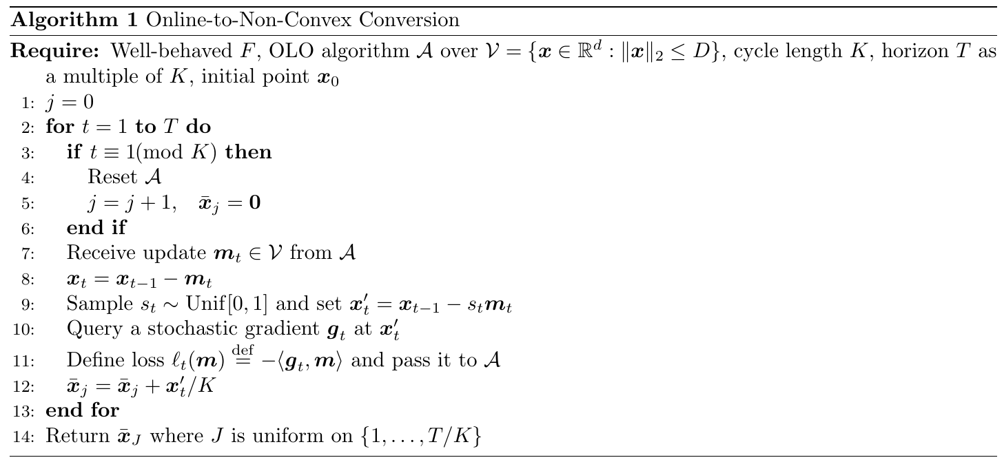
Remark 2. This notion is closely related to Goldstein-type ${\delta}$ -subdifferential stationarity, but we use gradients, and it is barycentric: the same convex weights used to average gradients must also average the sampled points back to ${{\boldsymbol x}}$ .

1.1. The Reduction Algorithm

We now present the reduction from non-convex optimization of well-behaved functions to online linear optimization.

Fix a cycle length ${K\in{\mathbb N}}$ and a radius ${D>0}$ . We will run an OLO algorithm ${\mathcal{A}}$ on the Euclidean ball ${\mathcal{V} = \{{\boldsymbol x}\in{\mathbb R}^d:\|{\boldsymbol x}\|_2\le D\}}$ , where the OLO algorithm outputs updates ${{\boldsymbol m}_t\in\mathcal{V}}$ . The iterates are defined by ${{\boldsymbol x}_{t}={\boldsymbol x}_{t-1}-{\boldsymbol m}_t}$ . Then, at each step we draw a random point ${{\boldsymbol x}'_{t}}$ on the segment from ${{\boldsymbol x}_{t-1}}$ to ${{\boldsymbol x}_{t}}$ and query a stochastic gradient there. The final output ${\bar{{\boldsymbol x}}_J}$ is the average of ${K}$ points ${{\boldsymbol x}'_{t}}$ inside a random cycle ${J}$ . The complete procedure is given in Algorithm 1.

Theorem 3. Let ${F}$ be well-behaved (Definition 1). Let ${\mathcal{F}_t}$ be the sigma-field generated by all randomness up to round ${t}$ before querying ${{\boldsymbol g}_t}$ , so that ${{\boldsymbol x}'_t}$ is ${\mathcal{F}_t}$ -measurable. With the notation in Algorithm 1, we assume

$\displaystyle \label{eq:stoch-oracle} \mathop{\mathbb E}[{\boldsymbol g}_t\mid \mathcal{F}_t]=\nabla F({\boldsymbol x}'_t), \qquad \mathop{\mathbb E}[\|{\boldsymbol g}_t\|_2^2\mid \mathcal{F}_t]\le G^2, \ \ \ \ \ (2)$

for some ${G>0}$ . Let ${T\in {\mathbb N}}$ be a multiple of the cycle length ${K}$ . Run Algorithm 1 for ${T}$ steps with cycle length ${K}$ , and instantiate ${\mathcal{A}}$ as projected \ac{OGD} over ${\mathcal{V}=\{{\boldsymbol x}\in{\mathbb R}^d:\|{\boldsymbol x}\|_2\le D\}}$ with learning rate ${\eta=D/(G\sqrt{K})}$ and initial point equal to ${\boldsymbol{0}}$ on each cycle (i.e., after each reset). Then,

$\displaystyle \mathop{\mathbb E}\left[ \frac{1}{T/K}\sum_{j=1}^{T/K} \left\|\frac{1}{K}\sum_{t=(j-1)K+1}^{jK}\nabla F({\boldsymbol x}'_t)\right\|_2 \right] \le \frac{F({\boldsymbol x}_0)-\inf_{{\boldsymbol x}} F({\boldsymbol x})}{D\,T} + \frac{2G}{\sqrt{K}}~.$

In particular, for ${\delta>0}$ , choose ${D=\delta/K}$ and then set

$\displaystyle K \asymp \left(\frac{G \, T \, \delta}{F({\boldsymbol x}_0)-\inf_{{\boldsymbol x}} F({\boldsymbol x})}\right)^{2/3}~,$

rounded to an integer. Then,

$\displaystyle \mathop{\mathbb E}\big[\|\nabla F(\bar{{\boldsymbol x}}_J)\|_\delta\big] = \mathcal{O}\left(G^\frac{2}{3}\,\left(\frac{F({\boldsymbol x}_0)-\inf_{{\boldsymbol x}} F({\boldsymbol x})}{T\delta}\right)^{1/3}\right)~.$

Proof: We first prove the key identity linking change in function value to an expected gradient. By Definition 1, we have

$\displaystyle \begin{aligned} F({\boldsymbol x}_{t})-F({\boldsymbol x}_{t-1}) &= \int_0^1 \! \langle\nabla F({\boldsymbol x}_{t-1}+a({\boldsymbol x}_{t}-{\boldsymbol x}_{t-1})),{\boldsymbol x}_{t}-{\boldsymbol x}_{t-1}\rangle\,\mathrm{d}a = \int_0^1 \! \langle\nabla F({\boldsymbol x}_{t-1}-a {\boldsymbol m}_{t}),-{\boldsymbol m}_{t}\rangle\,\mathrm{d}a\\ &=-\left\langle \mathop{\mathbb E}_{s_t}\big[\nabla F({\boldsymbol x}_{t-1}-s_t {\boldsymbol m}_{t})\big],{\boldsymbol m}_{t}\right\rangle =-\left\langle \mathop{\mathbb E}_{s_t}\big[\nabla F({\boldsymbol x}'_{t})\big],{\boldsymbol m}_{t}\right\rangle, \end{aligned}$

where the second to last equality is due to the fact that ${s_t}$ is uniform on ${[0,1]}$ .

Taking expectation over all randomness up to time ${t}$ (including ${s_t}$ ) and for any ${{\boldsymbol u}_j \in \mathcal{V}}$ , we have

$\displaystyle \begin{aligned} \mathop{\mathbb E}\left[F({\boldsymbol x}_t)-F({\boldsymbol x}_{t-1})\right] &= -\mathop{\mathbb E}\left[\langle\nabla F({\boldsymbol x}'_t),{\boldsymbol m}_t\rangle\right] \\ &= \mathop{\mathbb E}\left[\langle-{\boldsymbol g}_t,{\boldsymbol m}_t-{\boldsymbol u}_j\rangle\right] +\mathop{\mathbb E}\left[\langle{\boldsymbol g}_t-\nabla F({\boldsymbol x}'_t),{\boldsymbol m}_t\rangle\right] -\mathop{\mathbb E}\left[\langle{\boldsymbol g}_t,{\boldsymbol u}_j\rangle\right] \\ &= \mathop{\mathbb E}\left[\langle-{\boldsymbol g}_t,{\boldsymbol m}_t-{\boldsymbol u}_j\rangle\right] -\mathop{\mathbb E}\left[\langle{\boldsymbol g}_t,{\boldsymbol u}_j\rangle\right], \\ &= \mathop{\mathbb E}\left[\langle-{\boldsymbol g}_t,{\boldsymbol m}_t-{\boldsymbol u}_j\rangle\right] +\mathop{\mathbb E}\left[\langle-\nabla F({\boldsymbol x}'_t),{\boldsymbol u}_j\rangle\right]+\mathop{\mathbb E}\left[\langle\nabla F({\boldsymbol x}'_t)-{\boldsymbol g}_t,{\boldsymbol u}_j\rangle\right], & (3) \\\end{aligned}$

where in the second to last equality we used that ${{\boldsymbol m}_t}$ is determined before querying ${{\boldsymbol g}_t}$ , together with the unbiasedness condition ${\mathop{\mathbb E}[{\boldsymbol g}_t \mid \mathcal{F}_t] = \nabla F({\boldsymbol x}'_t)}$ .

We now analyze one cycle, and then sum over cycles. Fix a cycle ${j}$ and let its time indices be ${t=(j-1)K+1, \dots, jK}$ . Summing (3) over ${t=(j-1)K+1, \dots, jK}$ , we obtain

$\displaystyle \begin{aligned} \mathop{\mathbb E}\left[F({\boldsymbol x}_{jK})-F({\boldsymbol x}_{(j-1)K})\right] &= \mathop{\mathbb E}\left[\sum_{t=(j-1)K+1}^{jK}\langle -{\boldsymbol g}_t,{\boldsymbol m}_t-{\boldsymbol u}_j\rangle\right] - \mathop{\mathbb E}\left[\sum_{t=(j-1)K+1}^{jK} \langle\nabla F({\boldsymbol x}'_t),{\boldsymbol u}_j\rangle\right] \\ &\quad + \mathop{\mathbb E}\left[\sum_{t=(j-1)K+1}^{jK} \langle\nabla F({\boldsymbol x}'_t)-{\boldsymbol g}_t,{\boldsymbol u}_j\rangle\right]~. & (4) \\\end{aligned}$

We now focus on each term on the r.h.s. of this equality.

For the first term on the r.h.s. of (4), for any ${{\boldsymbol u}_j\in\mathcal{V}}$ , from the regret guarantee of projected Online Gradient Descent (OGD) with learning rate ${\eta=D/(G\sqrt{K})}$ and initial point equal to ${\boldsymbol{0}}$ , we have

$\displaystyle \begin{aligned} \sum_{t=(j-1)K+1}^{jK}\langle -{\boldsymbol g}_t,{\boldsymbol m}_t-{\boldsymbol u}_j\rangle &\leq \frac{\|{\boldsymbol u}_j\|_2^2}{2\eta} + \frac{\eta}{2} \sum_{t=(j-1)K+1}^{jK} \|{\boldsymbol g}_t\|_2^2 \leq \frac{D^2}{2\eta} + \frac{\eta}{2} \sum_{t=(j-1)K+1}^{jK} \|{\boldsymbol g}_t\|_2^2~. \end{aligned}$

Since this inequality holds for every ${{\boldsymbol u}_j}$ , we can use a hindsight choice depending on the gradients in cycle ${j}$ . Moreover, taking expectation and using the definition of ${\eta}$ , we have

$\displaystyle \mathop{\mathbb E}\left[\sum_{t=(j-1)K+1}^{jK}\langle -{\boldsymbol g}_t,{\boldsymbol m}_t-{\boldsymbol u}_j\rangle\right] \leq \frac{D^2}{2\eta} + \frac{\eta}{2} K G^2 = D G \sqrt{K}~. \label{eq:proof_non_convex_conversion_eq1} \ \ \ \ \ (5)$

Now, we choose ${{\boldsymbol u}_j}$ as

$\displaystyle {\boldsymbol u}_j \stackrel{\text{def}}{=} D\,\frac{\sum_{t=(j-1)K+1}^{jK}\nabla F({\boldsymbol x}'_t)}{\left\|\sum_{t=(j-1)K+1}^{jK}\nabla F({\boldsymbol x}'_t)\right\|_2} \quad \text{(and } {\boldsymbol u}_j=\boldsymbol{0} \text{ if the numerator is } \boldsymbol{0}\text{)}~.$

Our choice of ${{\boldsymbol u}_j}$ guarantees ${\|{\boldsymbol u}_j\|_2\le D}$ , so the second term of the r.h.s. of (4) becomes

$\displaystyle \mathop{\mathbb E}\left[\sum_{t=(j-1)K+1}^{jK}\langle\nabla F({\boldsymbol x}'_t),{\boldsymbol u}_j\rangle\right] = D\mathop{\mathbb E}\left[\left\|\sum_{t=(j-1)K+1}^{jK}\nabla F({\boldsymbol x}'_t)\right\|_2\right]~.$

Now, we upper bound the last term in (4). First, observe that

$\displaystyle \mathop{\mathbb E}[\|{\boldsymbol g}_t-\nabla F({\boldsymbol x}'_t)\|_2^2|\mathcal{F}_t] = \mathop{\mathbb E}[\|{\boldsymbol g}_t\|_2^2|\mathcal{F}_t]-\|\nabla F({\boldsymbol x}'_t)\|_2^2 \leq G^2,$

and

$\displaystyle \mathop{\mathbb E}[\langle{\boldsymbol g}_t-\nabla F({\boldsymbol x}'_t),{\boldsymbol g}_n-\nabla F({\boldsymbol x}'_n)\rangle |\mathcal{F}_t]=0, \quad \forall n< t~.$

Hence, we have

$\displaystyle \begin{aligned} \mathop{\mathbb E}\left[\sum_{t=(j-1)K+1}^{jK} \langle\nabla F({\boldsymbol x}'_t)-{\boldsymbol g}_t,{\boldsymbol u}_j\rangle\right] &\leq D \mathop{\mathbb E}\left[\left\|\sum_{t=(j-1)K+1}^{jK} ({\boldsymbol g}_t-\nabla F({\boldsymbol x}'_t))\right\|_2\right] \\ &\leq D\sqrt{\mathop{\mathbb E}\left[\left\|\sum_{t=(j-1)K+1}^{jK} ({\boldsymbol g}_t-\nabla F({\boldsymbol x}'_t))\right\|^2_2\right]}\\ &= D\sqrt{\mathop{\mathbb E}\left[\sum_{t=(j-1)K+1}^{jK} \|{\boldsymbol g}_t-\nabla F({\boldsymbol x}'_t)\|^2_2\right]}\\ &\leq G D\sqrt{K}, \end{aligned}$

where we used Cauchy–Schwarz’s inequality and Jensen’s inequality.

Putting everything together, we have

$\displaystyle D \, \mathop{\mathbb E}\left[\left\|\sum_{t=(j-1)K+1}^{jK}\nabla F({\boldsymbol x}'_t)\right\|_2\right] \le 2DG\sqrt{K} + \mathop{\mathbb E}\left[F({\boldsymbol x}_{(j-1)K})-F({\boldsymbol x}_{jK})\right]~.$

Summing over ${j=1,\dots,T/K}$ telescopes the function values:

$\displaystyle D\sum_{j=1}^{T/K} \mathop{\mathbb E}\left[\left\|\sum_{t=(j-1)K+1}^{jK}\nabla F({\boldsymbol x}'_t)\right\|_2\right] \le 2\frac{T}{K}\,DG\sqrt{K} + F({\boldsymbol x}_0)-\mathop{\mathbb E}[F({\boldsymbol x}_T)] \le 2\frac{T}{K}\,DG\sqrt{K} + F({\boldsymbol x}_0)-\inf_{{\boldsymbol x}} F({\boldsymbol x})~.$

Dividing by ${DT}$ gives the stated bound.

Now observe that within each cycle we have ${\|{\boldsymbol x}_t-{\boldsymbol x}_{t-1}\|_2=\|{\boldsymbol m}_t\|_2\le D}$ . Hence all points ${{\boldsymbol x}'_t}$ lie in the convex hull of ${\{{\boldsymbol x}_{(j-1)K},{\boldsymbol x}_{(j-1)K+1},\dots,{\boldsymbol x}_{jK}\}}$ whose diameter is at most ${KD}$ (triangle inequality over at most ${K}$ steps). Since ${\bar{{\boldsymbol x}}_j=\frac1K\sum_{t=(j-1)K+1}^{jK}{\boldsymbol x}'_t}$ , every ${{\boldsymbol x}'_t}$ lies at distance at most the diameter of the set from ${\bar{{\boldsymbol x}}_j}$ , i.e., ${KD}$ . Therefore, if ${D=\delta/K}$ , then for all ${t}$ in cycle ${j}$ we have ${{\boldsymbol x}'_t \in \mathcal{B}(\bar{{\boldsymbol x}}_j,\delta)}$ . By Definition 2,

$\displaystyle \|\nabla F(\bar{{\boldsymbol x}}_j)\|_\delta \le \left\|\frac{1}{K}\sum_{t=(j-1)K+1}^{jK}\nabla F({\boldsymbol x}'_t)\right\|_2~.$

Sampling ${J}$ uniformly over cycles and taking expectation yields the stated barycentric ${(\delta,\epsilon)}$ -stationarity bound. Choosing ${K}$ to balance the two terms (with ${D=\delta/K}$ ) gives the stated rate. $\Box$

It is interesting to compute the update ${{\boldsymbol m}_t}$ in Algorithm 1 when ${\mathcal{A}}$ is projected OGD:

$\displaystyle {\boldsymbol m}_{t+1} = \Pi_{\mathcal{V}}({\boldsymbol m}_{t} + \eta {\boldsymbol g}_t)~.$

This is reminiscent of the Stochastic Gradient Descent (SGD) update with momentum and clipping, which are common heuristics for optimizing non-convex objectives in deep learning. Yet, here the update comes naturally from the theory.

We can also prove that this bound is optimal. To see this, we consider smooth functions and the following lemma.

Lemma 4. Suppose that ${F:{\mathbb R}^d \rightarrow {\mathbb R}}$ is ${H}$ -smooth and ${{\boldsymbol x}}$ satisfies ${\|\nabla F ({\boldsymbol x})\|_\delta \leq \epsilon}$ . Then, ${\|\nabla F({\boldsymbol x})\|_2 \leq \epsilon + H\delta}$ .

Proof: Since ${\|\nabla F({\boldsymbol x})\|_\delta\leq \epsilon}$ , for any ${p>0}$ there exists ${Q\in\mathcal{Q}({\boldsymbol x},\delta)}$ such that ${\left\|\mathop{\mathbb E}_{{\boldsymbol y}\sim Q}[\nabla F({\boldsymbol y})]\right\|_2 \leq \epsilon + p}$ .

By definition of ${\mathcal{Q}({\boldsymbol x},\delta)}$ , we have ${\text{supp}(Q)\subseteq \mathcal{B}({\boldsymbol x},\delta)}$ . So, by ${H}$ -smoothness, for every ${{\boldsymbol y}\in\text{supp}(Q)}$ , we have ${\|\nabla F({\boldsymbol y})-\nabla F({\boldsymbol x})\|_2 \leq H\|{\boldsymbol y}-{\boldsymbol x}\|_2 \leq H\delta}$ . Hence,

$\displaystyle \begin{aligned} \epsilon + p & \geq \left\|\mathop{\mathbb E}_{{\boldsymbol y}\sim Q}[\nabla F({\boldsymbol y})]\right\|_2 = \left\|\nabla F({\boldsymbol x}) + \mathop{\mathbb E}_{{\boldsymbol y}\sim Q}\big[\nabla F({\boldsymbol y})-\nabla F({\boldsymbol x})\big]\right\|_2 \\ &\geq \|\nabla F({\boldsymbol x})\|_2 - \left\|\mathop{\mathbb E}_{{\boldsymbol y}\sim Q}\big[\nabla F({\boldsymbol y})-\nabla F({\boldsymbol x})\big]\right\|_2 \\ &\geq \|\nabla F({\boldsymbol x})\|_2 - \mathop{\mathbb E}_{{\boldsymbol y}\sim Q}\left[\|\nabla F({\boldsymbol y})-\nabla F({\boldsymbol x})\|_2\right] \\ &\geq \|\nabla F({\boldsymbol x})\|_2 - H\delta~. \end{aligned}$

Therefore, ${\|\nabla F({\boldsymbol x})\|_2 \leq \epsilon + H\delta + p}$ . Since this holds for every ${p>0}$ , we conclude that ${\|\nabla F({\boldsymbol x})\|_2 \leq \epsilon + H\delta}$ . $\Box$

Now, recall that Theorem 3 shows that we can find a ${(\delta, \epsilon)}$ barycentric stationary point in ${\mathcal{O}(\epsilon^{-3} \delta^{-1})}$ iterations. Thus, Lemma 4 implies that by setting ${\delta = \epsilon/H}$ , we can find an ${2\epsilon}$ -stationary point of an ${H}$ -smooth objective ${F}$ in ${\mathcal{O}(\epsilon^{-4})}$ iterations, which matches the optimal guarantee of standard SGD. Hence, the ${\mathcal{O}(\epsilon^{-3}\delta^{-1})}$ rate in Theorem 3 is optimal for all ${\epsilon}$ of the order of ${\delta H}$ .

2. History Bits

Zhang et al. (2020) proposed to use the Goldstein stationarity condition (Goldstein, 1977) for non-convex non-smooth objectives. They also proved a suboptimal bound of ${\mathcal{O}(\epsilon^{-4}\delta^{-1})}$ . The barycentric definition, Theorem 3, and Lemma 4 are from Cutkosky et al. (2023). Note that I changed Definition 2 a bit because Algorithm 1 can return repeated points, that would not be allowed by the original definition in Cutkosky et al. (2023). The barycentric part of the definition is not strictly necessary for the results I presented, yet it is necessary for the additional results in Cutkosky et al. (2023) on functions whose Hessian is Lipschitz. Zhang&Cutkosky (2024) improved the reduction in Algorithm 1 using an exponentially distributed ${s_t}$ , which allows one to query the gradient at ${{\boldsymbol x}_t}$ rather than at the intermediate point ${{\boldsymbol x}'_t}$ , and removes the feasible set ${\mathcal{V}}$ . Jordan et al. (2023) proved that the randomization is essential in this class of problems to achieve dimension-free rates.