In this post, we introduce yet another way to quantify the ability of online learning algorithms to compete with a different comparators, besides the dynamic regret that we saw last time.
1. Strongly Adaptive Regret
We introduce the concept of strongly adaptive regret:
This definition captures the fact that we want the performance of the algorithm to be good on any interval of length . We will say that the algorithm is strongly adaptive if the additional price we pay with respect to learning on any specific interval of length is at most polylogarithmic in .
Remark 1. One might be tempted to remove the dependency on and consider
This notion is known as adaptive regret. However, it is clear that for bounded domains and Lipschitz losses (from the OLO lower bound), that is meaningless for intervals of size . Hence, the adaptive regret does not allow us to reason on the performance of the algorithm on small intervals.
In the next section, we show how to obtain strongly adaptive algorithms, using once again a combination of online learning algorithms.
1.1. CBCE: A Meta Algorithm for Strongly Adaptive Regret
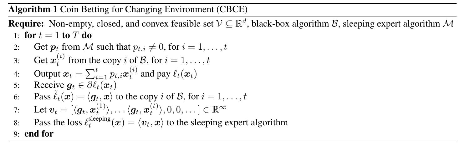
We will introduce now the Coin Betting for Changing Environment (CBCE) algorithm, see Algorithm 1. We use different OCO algorithms, each one starting at a different time step, and we combine them with a sleeping-experts algorithm over a countably infinite number of experts. In particular, is the output at time of the OCO algorithm started at time , while is the convex combination of using the probability distribution produced by the sleeping expert algorithm. Using the sleeping expert algorithm in Example 1 in the sleeping expert post, immediately gives the following theorem.
Theorem 1. Let a non-empty closed convex set. Let the algorithm in Example 1 in the sleeping expert post, where for , and an online learning algorithm that satisfies for all , where . Let . Then, Algorithm 1 satisfies
Proof: Like in the case of ADER, a simple implementation of this algorithm would require to query values of the function at time . However, we run the algorithm on the linearized losses , where , so that the subgradient is only asked once. Hence, we upper bound the regret using the linearized losses:
Next, we decompose the regret in the contributes of and as
The first sum can be written as
because the -th copy of the algorithm has been active only on rounds to . With the choice of , the sleeping expert algorithm in Example 1 in the sleeping expert post achieves a sleeping regret against the -th expert of , because the expert has been active for rounds. For the second sum, we simply have because the -th copy of algorithm was started on round .
Hence, assuming that , the CBCE algorithm is strongly adaptive because the regret on any interval of length depends on and only logarithmically on .
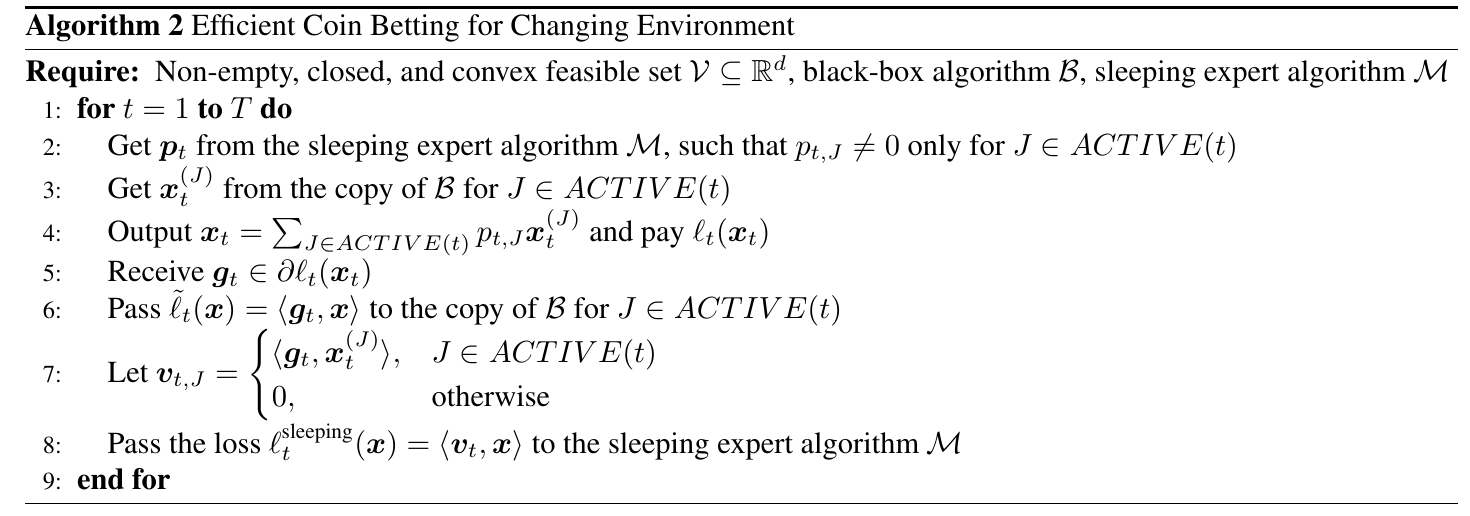
However, while we ask only one subgradient per round, the computational complexity of CBCE in round is proportional to , because we have to update OCO algorithms. So, in the next section, we consider an efficient variant of the CBCE algorithm, whose update is proportional to , with the same strongly adaptive regret guarantee.
1.2. Efficient Version of CBCE
The previous algorithm has the disadvantage of requiring to start a new copy of algorithm in each iteration. Instead, here we will see how to reduce the number of copies to the logarithm of the number of rounds, using geometric coverings.
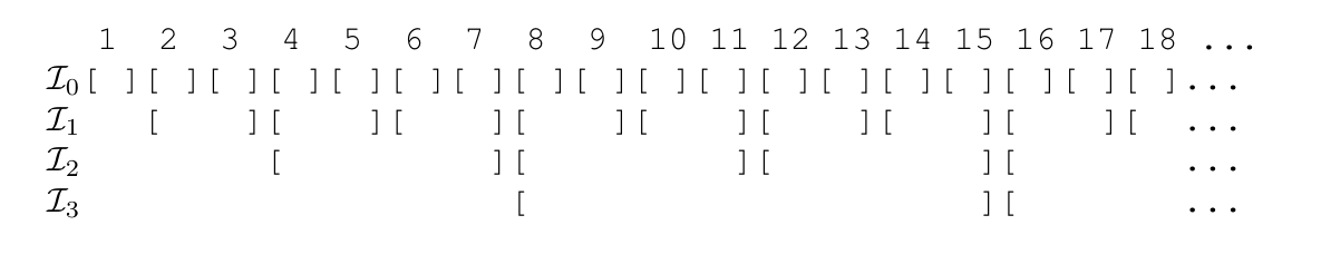
Figure 1. Geometric covering intervals. Each interval is denoted by [ ].
For , define the intervals
That is, each is a partition of to consecutive intervals of length . Also, define
and
the set of the “active” intervals at time , that is, the intervals that contain . By the definition of , for every we have that no interval in contains , while for every we have that a single interval in contains . Therefore, . We will run a copy of an OCO algorithm for each active interval, this means that we have a number of algorithms at each time step that is logarithmic in . Given an interval of , we will also use the definition of
to denote the set of the intervals in that contains a .
The next lemma allows to decompose the regret over any interval using the regret over intervals in .
Lemma 2. Let be an arbitrary interval. Then, the interval can be paritioned into two finite sequences of disjoint and consecutive intervals, denoted and , such that
.
.
Proof: The intuition of the proof is the following one: First, we choose the interval to be the biggest leftmost one in . Then, we show that the others are selected so that they decrease in size to the left, while on the right can have the same size of and the others will decrease in size.
Denote the size of by for and let be the maximal size of any interval that is contained in . Among all of these intervals, let be the leftmost interval, i.e., we define
Starting from , we now define a sequence of intervals (in a reversed order), denoted to cover the interval , as follows:
Clearly, this sequence is finite and the left endpoint of the leftmost interval, , is . Denote the size of by . We next prove that for every , . Given that the intervals are powers of 2, it suffices to show that for every . We use induction. The base case follows from the fact that , otherwise it would contradict the maximality of and the fact that is the leftmost biggest interval. We next assume that the claim holds for every and prove for . Assume by contradiction that . Consider the interval which is obtained by extending to its left by an additional size of , that is, . Hence, is an interval of size and it is contained in . According to the induction hypothesis, for some . Given that is adjacent to the interval and its size is for some , from the definition of , we have that , contradicting the maximality of .
Similarly, we define a sequence of disjoint and consecutive intervals, denoted that covers .
Clearly, this sequence is finite and the right endpoint of the rightmost interval, , is . Denote the size of by . We next prove that for every , that is equivalent to .
We prove it again by induction. We assume that for every and prove that for . For the base case, from the definition of we have that . Now, assume by contradiction that . Then, we can consider the interval which is obtained by extending to its right by an additional size of . It follows that is an interval of size and it is contained in . According to the induction hypothesis, for some . We need to consider the following two cases:
Case (i.e., ). Then, is consecutive to and its size is , hence , contradicting the maximality of .
Case (i.e., ). Then, and this contradicts the maximality of .
As an example of the above Lemma, consider the interval that is partitioned in the intervals , , , , , , , .
We will use an expert algorithm over a countable number of experts, hence we also have a prior over the infinite-dimensional simplex . For simplicity of notation, we denote by the elements of associated with the interval .
Theorem 3. Let a non-empty closed convex set. Let be the algorithm in Example 1 in the sleeping expert post, where the copy associated to the interval has the parameter defined recursively as
Let be an online learning algorithm that satisfies for all and , where . Let . Then, Algorithm 1 satisfies
Proof: First of all, we upper bound the regret over the interval with the one over linearized losses:
where .
Now, suppose we denote by the decision from the black-box run associated with the interval at time and by the combined decision of the meta algorithm at time . Since the complete algorithm is a combination of a meta algorithm and several black-box algorithms , its regret depends on both and . We now decompose the two sources of regret additively through the geometric covering.
Let be the partition of obtained from Lemma 2. Then, the regret on can be decomposed as follows:
The black-box regret on is exactly the regret of the black-box algorithm on rounds, since the black-box run was started at the beginning of the interval . In particular, we have
where the second inequality is due to Lemma 2 and in the last one we used that the number of geometric cover intervals is less than (again from Lemma 2) and .
Now, we show that has low regret on interval , considering separately the regret on for and . The critical observation is that
where the equality holds because the expert associated to is active only for the rounds in . Using the guarantee on the sleeping regret in Example 1 in the sleeping expert post, we have
where the second inequality is due to Lemma 2. Analogously, we have
Putting all together, we have the stated bound.
Remark 2. Observe that the limit for of the first term of the upper bound of the regret is . However, the second term is always of the order of .
From the above theorem, it is immediate to get a guarantee on the strongly adaptive regret by observing that
2. History Bits
The adaptive regret is defined in Hazan&Seshadhri (2007), Hazan&Seshadhri (2009). The strongly-adaptive regret was defined by Adamskiy et al. (2012), Adamskiy et al. (2016) (still calling it “adaptive regret”) and then reinvented in Daniely et al. (2015) (that coined the name). Note that the strongly-adaptive regret is usually defined for bounded domains, taking the maximum with respect , instead I defined it more generally for any competitor in the feasible set. Lemma 2 is from Daniely et al. (2015) as well. The efficient version of the CBCE algorithm was proposed by Jun et al. (2017), Jun et al. (2017) using a stronger version of the sleeping expert algorithm, still based on coin betting. I simplified the sleeping expert algorithm for didactical reasons. CBCE improves over the guarantee in Daniely et al. (2015) by improving the logarithmic term. The ideas of using linearized losses in CBCE to avoid querying more than one subgradients and the better behaviour of the first term in the bound when are new. The non-efficient version of CBCE is also new, but straightforward.
Acknowledgements
Thanks to Wei-Cheng Lee and Yulian Wu for feedback on this post.
![\displaystyle \text{SA-Regret}_{T,\tau}({\boldsymbol u}) :=\max_{[s,s+\tau-1] \subseteq [1,2,\dots, T]} \ \sum_{t=s}^{s+\tau-1} \ell_t({\boldsymbol x}_t) - \sum_{t=s}^{s+\tau-1} \ell_t({\boldsymbol u}), \ \forall {\boldsymbol u} \in \mathcal{V}~.](https://s0.wp.com/latex.php?latex=%5Cdisplaystyle+%5Ctext%7BSA-Regret%7D_%7BT%2C%5Ctau%7D%28%7B%5Cboldsymbol+u%7D%29+%3A%3D%5Cmax_%7B%5Bs%2Cs%2B%5Ctau-1%5D+%5Csubseteq+%5B1%2C2%2C%5Cdots%2C+T%5D%7D+%5C+%5Csum_%7Bt%3Ds%7D%5E%7Bs%2B%5Ctau-1%7D+%5Cell_t%28%7B%5Cboldsymbol+x%7D_t%29+-+%5Csum_%7Bt%3Ds%7D%5E%7Bs%2B%5Ctau-1%7D+%5Cell_t%28%7B%5Cboldsymbol+u%7D%29%2C+%5C+%5Cforall+%7B%5Cboldsymbol+u%7D+%5Cin+%5Cmathcal%7BV%7D%7E.+&bg=ffffff&fg=000000&s=0&c=20201002)


for bounded domains and Lipschitz losses (from the OLO lower bound), that is meaningless for intervals of size
. Hence, the adaptive regret does not allow us to reason on the performance of the algorithm on small intervals.


a non-empty closed convex set. Let
the algorithm in Example 1 in the sleeping expert post, where
for
, and
an online learning algorithm that satisfies
for all
, where
. Let
. Then, Algorithm 1 satisfies


![\displaystyle \mathcal{I}_k :=\{[i 2^k,(i+1)2^k-1] : i \in {\mathbb N}\}~.](https://s0.wp.com/latex.php?latex=%5Cdisplaystyle+%5Cmathcal%7BI%7D_k+%3A%3D%5C%7B%5Bi+2%5Ek%2C%28i%2B1%292%5Ek-1%5D+%3A+i+%5Cin+%7B%5Cmathbb+N%7D%5C%7D%7E.+&bg=ffffff&fg=000000&s=0&c=20201002)


be an arbitrary interval. Then, the interval
and
, such that
.
.


![\displaystyle \begin{aligned} q_0 &:= \mathop{\mathrm{argmin}}\{q': [q',q'+b_0-1]\in \mathcal{I}|_J\},\\ s_0 &:= q_0+b_0-1,\\ J_0 &:=[q_0,s_0]~. \end{aligned}](https://s0.wp.com/latex.php?latex=%5Cdisplaystyle+%5Cbegin%7Baligned%7D+q_0+%26%3A%3D+%5Cmathop%7B%5Cmathrm%7Bargmin%7D%7D%5C%7Bq%27%3A+%5Bq%27%2Cq%27%2Bb_0-1%5D%5Cin+%5Cmathcal%7BI%7D%7C_J%5C%7D%2C%5C%5C+s_0+%26%3A%3D+q_0%2Bb_0-1%2C%5C%5C+J_0+%26%3A%3D%5Bq_0%2Cs_0%5D%7E.+%5Cend%7Baligned%7D&bg=ffffff&fg=000000&s=0&c=20201002)


![{[1, q_0-1]}](https://s0.wp.com/latex.php?latex=%7B%5B1%2C+q_0-1%5D%7D&bg=ffffff&fg=000000&s=0&c=20201002)
![\displaystyle \begin{aligned} [q_{-1},s_{-1}] &:=J_{-1} :=\mathop{\mathrm{argmax}}_{J'=[q',s'] \in \mathcal{I}|_{[q,q_0-1]}: s'=q_0-1} |J'|\\ &\vdots\\ [q_{-i},s_{-i}] &:=J_{-i} :=\mathop{\mathrm{argmax}}_{J'=[q',s'] \in \mathcal{I}|_{[q,q_{i+1}-1]}: s'=q_{-i+1}-1} |J'|\\ &\vdots \end{aligned}](https://s0.wp.com/latex.php?latex=%5Cdisplaystyle+%5Cbegin%7Baligned%7D+%5Bq_%7B-1%7D%2Cs_%7B-1%7D%5D+%26%3A%3DJ_%7B-1%7D+%3A%3D%5Cmathop%7B%5Cmathrm%7Bargmax%7D%7D_%7BJ%27%3D%5Bq%27%2Cs%27%5D+%5Cin+%5Cmathcal%7BI%7D%7C_%7B%5Bq%2Cq_0-1%5D%7D%3A+s%27%3Dq_0-1%7D+%7CJ%27%7C%5C%5C+%26%5Cvdots%5C%5C+%5Bq_%7B-i%7D%2Cs_%7B-i%7D%5D+%26%3A%3DJ_%7B-i%7D+%3A%3D%5Cmathop%7B%5Cmathrm%7Bargmax%7D%7D_%7BJ%27%3D%5Bq%27%2Cs%27%5D+%5Cin+%5Cmathcal%7BI%7D%7C_%7B%5Bq%2Cq_%7Bi%2B1%7D-1%5D%7D%3A+s%27%3Dq_%7B-i%2B1%7D-1%7D+%7CJ%27%7C%5C%5C+%26%5Cvdots+%5Cend%7Baligned%7D&bg=ffffff&fg=000000&s=0&c=20201002)


![{\hat{J}_{-n+1}:=[q_{-n+1}-b_{-n+1},q_{-n+1}-1]\cup J_{-n+1}}](https://s0.wp.com/latex.php?latex=%7B%5Chat%7BJ%7D_%7B-n%2B1%7D%3A%3D%5Bq_%7B-n%2B1%7D-b_%7B-n%2B1%7D%2Cq_%7B-n%2B1%7D-1%5D%5Ccup+J_%7B-n%2B1%7D%7D&bg=ffffff&fg=000000&s=0&c=20201002)


![{[s_0 + 1, s]}](https://s0.wp.com/latex.php?latex=%7B%5Bs_0+%2B+1%2C+s%5D%7D&bg=ffffff&fg=000000&s=0&c=20201002)
![\displaystyle \begin{aligned} [q_{1},s_{1}] &:=J_{1} :=\mathop{\mathrm{argmax}}_{J'=[q',s'] \in \mathcal{I}|_{[s_0+1,s]}: q'=s_0+1} |J'|\\ &\vdots\\ [q_{i},s_{i}] &:=J_{i} :=\mathop{\mathrm{argmax}}_{J'=[q',s'] \in \mathcal{I}|_{[s_{i-1}+1,s]}: q'=s_{i-1}+1} |J'|\\ &\vdots \end{aligned}](https://s0.wp.com/latex.php?latex=%5Cdisplaystyle+%5Cbegin%7Baligned%7D+%5Bq_%7B1%7D%2Cs_%7B1%7D%5D+%26%3A%3DJ_%7B1%7D+%3A%3D%5Cmathop%7B%5Cmathrm%7Bargmax%7D%7D_%7BJ%27%3D%5Bq%27%2Cs%27%5D+%5Cin+%5Cmathcal%7BI%7D%7C_%7B%5Bs_0%2B1%2Cs%5D%7D%3A+q%27%3Ds_0%2B1%7D+%7CJ%27%7C%5C%5C+%26%5Cvdots%5C%5C+%5Bq_%7Bi%7D%2Cs_%7Bi%7D%5D+%26%3A%3DJ_%7Bi%7D+%3A%3D%5Cmathop%7B%5Cmathrm%7Bargmax%7D%7D_%7BJ%27%3D%5Bq%27%2Cs%27%5D+%5Cin+%5Cmathcal%7BI%7D%7C_%7B%5Bs_%7Bi-1%7D%2B1%2Cs%5D%7D%3A+q%27%3Ds_%7Bi-1%7D%2B1%7D+%7CJ%27%7C%5C%5C+%26%5Cvdots+%5Cend%7Baligned%7D&bg=ffffff&fg=000000&s=0&c=20201002)


(i.e.,
). Then,
and its size is
, hence
, contradicting the maximality of
(i.e.,
). Then,
and this contradicts the maximality of
.
![{J=[1,30]}](https://s0.wp.com/latex.php?latex=%7BJ%3D%5B1%2C30%5D%7D&bg=ffffff&fg=000000&s=0&c=20201002)
![{J_{-3}=[1]}](https://s0.wp.com/latex.php?latex=%7BJ_%7B-3%7D%3D%5B1%5D%7D&bg=ffffff&fg=000000&s=0&c=20201002)
![{J_{-2}=[2,3]}](https://s0.wp.com/latex.php?latex=%7BJ_%7B-2%7D%3D%5B2%2C3%5D%7D&bg=ffffff&fg=000000&s=0&c=20201002)
![{J_{-1}=[4,7]}](https://s0.wp.com/latex.php?latex=%7BJ_%7B-1%7D%3D%5B4%2C7%5D%7D&bg=ffffff&fg=000000&s=0&c=20201002)
![{J_{0}=[8,15]}](https://s0.wp.com/latex.php?latex=%7BJ_%7B0%7D%3D%5B8%2C15%5D%7D&bg=ffffff&fg=000000&s=0&c=20201002)
![{J_1=[16,23]}](https://s0.wp.com/latex.php?latex=%7BJ_1%3D%5B16%2C23%5D%7D&bg=ffffff&fg=000000&s=0&c=20201002)
![{J_2=[24,27]}](https://s0.wp.com/latex.php?latex=%7BJ_2%3D%5B24%2C27%5D%7D&bg=ffffff&fg=000000&s=0&c=20201002)
![{J_3=[28,29]}](https://s0.wp.com/latex.php?latex=%7BJ_3%3D%5B28%2C29%5D%7D&bg=ffffff&fg=000000&s=0&c=20201002)
![{J_4=[30]}](https://s0.wp.com/latex.php?latex=%7BJ_4%3D%5B30%5D%7D&bg=ffffff&fg=000000&s=0&c=20201002)


has the parameter
defined recursively as
for all
and
. Let


![{i\in [-a,0]}](https://s0.wp.com/latex.php?latex=%7Bi%5Cin+%5B-a%2C0%5D%7D&bg=ffffff&fg=000000&s=0&c=20201002)
![{i \in [1,b]}](https://s0.wp.com/latex.php?latex=%7Bi+%5Cin+%5B1%2Cb%5D%7D&bg=ffffff&fg=000000&s=0&c=20201002)


of the first term of the upper bound of the regret is
. However, the second term is always of the order of

