Black-Box Reductions: Constrained Online Learning

This is the first post on a new topic: how to reduce one online learning problem into another in a black-box way. That is, we will use an online convex optimization algorithm to solve a problem different from what it was meant to solve, without looking at its internal working in any way. The only thing we will change will be the input we pass to the algorithm. Why doing it? Because you might have optimization software that you cannot modify or just because designing and analyzing an online learning algorithm in one case might be easier.

Here, I’ll explain how to deal with constraints in online convex optimization in a black box way, and as a bonus, I’ll show how to easily prove the regret guarantee of the Regret Matching+ algorithm.

1. Solving Constrained OCO

We might have an Online Convex Optimization (OCO) algorithm designed for constrained online linear optimization over a feasible set ${W \subseteq {\mathbb R}^d}$ and we might wonder how we can use it for online convex optimization on a feasible set ${V\subset W}$ . How do we deal with the smaller feasible set?

Let’s see a prototypical example of this approach. We have a OCO algorithm that outputs in each round ${{\boldsymbol z}_t \in W={\mathbb R}^d_{\geq 0}}$ and we want to use it for OCO in ${V=\Delta^{d-1}}$ . So, first of all, we have to transform ${{\boldsymbol z}_t}$ into a vector of the probability simplex. One way to do it could be to normalize it by its L1 norm. So, we predict in each round by ${{\boldsymbol x}_t=\frac{{\boldsymbol z}_t}{\|{\boldsymbol z}_t\|_1}}$ if ${\|{\boldsymbol z}_t\|_1\neq 0}$ and with any other vector in the simplex if ${\|{\boldsymbol z}_t\|_1=0}$ . Now, we have to find a way to penalize the algorithm every time its prediction is outside ${V}$ , for example passing to it a surrogate loss. In formulas, we have

$\displaystyle \begin{aligned} \text{Regret}_T({\boldsymbol u}) &= \sum_{t=1}^T(\ell_t({\boldsymbol x}_t)-\ell_t({\boldsymbol u})) \leq \sum_{t=1}^T \langle {\boldsymbol g}_t, {\boldsymbol x}_t-{\boldsymbol u}\rangle \nonumber \\ &= \sum_{t=1}^T (\langle {\boldsymbol g}_t, {\boldsymbol z}_t-{\boldsymbol u}\rangle + \langle {\boldsymbol g}_t, {\boldsymbol x}_t-{\boldsymbol z}_t\rangle), \end{aligned}$

where ${{\boldsymbol g}_t \in \partial \ell_t({\boldsymbol x}_t)}$ . Now, we want to find ${\hat{{\boldsymbol g}}_t}$ such that

$\displaystyle \langle {\boldsymbol g}_t, {\boldsymbol x}_t-{\boldsymbol z}_t\rangle \leq \langle \hat{{\boldsymbol g}}_t, {\boldsymbol z}_t-{\boldsymbol u}\rangle, \ \forall {\boldsymbol u} \in V~.$

If we could do it, we would have

$\displaystyle \begin{aligned} \text{Regret}_T({\boldsymbol u}) &\leq \sum_{t=1}^T \langle {\boldsymbol g}_t+ \hat{{\boldsymbol g}}_t, {\boldsymbol z}_t-{\boldsymbol u}\rangle, \end{aligned}$

that is the regret of the OCO algorithm on some surrogate linear losses.

Using our definition of ${{\boldsymbol x}_t}$ , we have that if ${\|{\boldsymbol z}_t\|_1\neq 0}$ then

$\displaystyle \langle {\boldsymbol g}_t, {\boldsymbol x}_t-{\boldsymbol z}_t\rangle = \left\langle {\boldsymbol g}_t, \frac{{\boldsymbol z}_t}{\|{\boldsymbol z}_t\|_1}-{\boldsymbol z}_t\right\rangle = \left\langle {\boldsymbol g}_t, \frac{{\boldsymbol z}_t}{\|{\boldsymbol z}_t\|_1}\right\rangle \left(1-\|{\boldsymbol z}_t\|_1\right) = -\langle {\boldsymbol g}_t, {\boldsymbol x}_t\rangle \langle [1, \dots ,1]^\top, {\boldsymbol z}_t - {\boldsymbol u} \rangle~.$

Instead, if ${\|{\boldsymbol z}_t\|_1=0}$ we have

$\displaystyle \langle {\boldsymbol g}_t, {\boldsymbol x}_t-{\boldsymbol z}_t\rangle = \langle {\boldsymbol g}_t, {\boldsymbol x}_t\rangle = -\langle {\boldsymbol g}_t, {\boldsymbol x}_t\rangle \langle [1, \dots ,1]^\top, {\boldsymbol z}_t - {\boldsymbol u} \rangle~.$

Hence, we have that ${\hat{{\boldsymbol g}_t}=- \langle {\boldsymbol g}_t, {\boldsymbol x}_t\rangle [1, \dots, 1]^\top}$ and the surrogate linear losses we will pass to the OCO algorithm are

$\displaystyle \label{eq:constrained_reduction_old} \tilde{\ell}_t({\boldsymbol x})=\langle {\boldsymbol g}_t - [1, \dots, 1]^\top \langle {\boldsymbol g}_t, {\boldsymbol x}_t\rangle,{\boldsymbol x}\rangle~. \ \ \ \ \ (1)$

In this way, we have

$\displaystyle \text{Regret}_T({\boldsymbol u}) = \sum_{t=1}^T(\ell_t({\boldsymbol x}_t)-\ell_t({\boldsymbol u})) \leq \sum_{t=1}^T(\tilde{\ell}_t({\boldsymbol z}_t)-\tilde{\ell}_t({\boldsymbol u}))~.$

It is worth noting that the norm of the gradients of the surrogate losses is controlled: ${\|{\boldsymbol g}_t-[1, \dots, 1]^\top \langle {\boldsymbol g}_t, {\boldsymbol x}_t\rangle\|_\infty\leq 2\|{\boldsymbol g}_t\|_\infty}$ .

We solved our problem, but this approach does not seem to scale to arbitrary complex feasible sets. Hence, we need a more general way to solve it. In the following, we will show two complementary ways to do it.

1.1. Dealing with Constraints using (Non-Euclidean) Projections

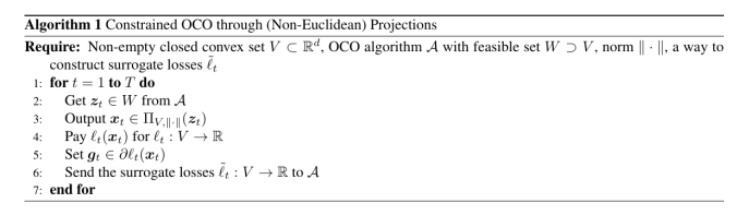
Now, we extend the procedure in the previous section to general convex sets and general norms. First of all, we need some definitions and basic results.

Definition 1 (Distance to a set ${V}$ and generalized projection). Let ${V\subset {\mathbb R}^d}$ be a convex and closed set. The distance to a set with respect to the norm ${\|\cdot\|}$ is the function ${\text{dist}_{V,\|\cdot\|}:{\mathbb R}^d \rightarrow {\mathbb R}}$ defined as ${\text{dist}_{V,\|\cdot\|}({\boldsymbol x})=\min_{{\boldsymbol y} \in V} \|{\boldsymbol x}-{\boldsymbol y}\|}$ . We also define the generalized projection function ${\Pi_{V, \|\cdot\|}: {\mathbb R}^d \rightarrow {\mathbb R}^d}$ defined as ${\Pi_{V, \|\cdot\|} \in \mathop{\mathrm{argmin}}_{{\boldsymbol y} \in V} \ \|{\boldsymbol x}-{\boldsymbol y}\|}$ .

We have the following properties for the distance to a set function.

Lemma 2. Let ${V}$ convex and closed. Then, we have

${\text{dist}_{V, \|\cdot\|}}$ is convex.

${\text{dist}_{V, \|\cdot\|}}$ is 1-Lipschitz with respect to ${\|\cdot\|_\star}$ .

${\partial \text{dist}_{V,\|\cdot\|}({\boldsymbol x}) = \begin{cases} \{{\boldsymbol g}\} & {\boldsymbol x} \notin V\\ \{\boldsymbol{0}\}, & {\boldsymbol x} \in V \end{cases}}$ , where ${\|{\boldsymbol g}\|_\star=1}$ and ${\|{\boldsymbol x}-\Pi_{V,\|\cdot\|}({\boldsymbol x})\|= \langle {\boldsymbol g}, {\boldsymbol x}-\Pi_{V,\|\cdot\|}({\boldsymbol x})\rangle}$ .

Proof: For the first property, we have

$\displaystyle \begin{aligned} \text{dist}_{V,\|\cdot\|}(\lambda {\boldsymbol x} + (1-\lambda) {\boldsymbol z}) &= \min_{{\boldsymbol y} \in V} \| \lambda {\boldsymbol x} + (1-\lambda) {\boldsymbol z} - {\boldsymbol y}\| \leq \| \lambda {\boldsymbol x} + (1-\lambda) {\boldsymbol z} - (\lambda \Pi_{V,\|\cdot\|}({\boldsymbol x}) + (1-\lambda) \Pi_{V,\|\cdot\|}({\boldsymbol z})\| \\ &= \|\lambda ({\boldsymbol x}-\Pi_{V,\|\cdot\|}({\boldsymbol x})) + (1-\lambda)({\boldsymbol z}-\Pi_{V,\|\cdot\|}({\boldsymbol z}))\| \leq \lambda \text{dist}_{V,\|\cdot\|}({\boldsymbol x}) + (1-\lambda) \text{dist}_{V,\|\cdot\|}({\boldsymbol z}), \end{aligned}$

where in the first inequality we used the convexity of ${V}$ .

For the second property, we have that

$\displaystyle \begin{aligned} \text{dist}_{V,\|\cdot\|}({\boldsymbol x}+{\boldsymbol \delta}) - \text{dist}_{V,\|\cdot\|}({\boldsymbol x}) &= \min_{{\boldsymbol y} \in V} \ \|{\boldsymbol x} + {\boldsymbol \delta} - {\boldsymbol y}\| - \|{\boldsymbol x} - \Pi_{V,\|\cdot\|}({\boldsymbol x})\| \leq \|{\boldsymbol x} + {\boldsymbol \delta} - \Pi_{V,\|\cdot\|}({\boldsymbol x})\| - \|{\boldsymbol x} - \Pi_{V,\|\cdot\|}({\boldsymbol x})\| \\ &\leq \|{\boldsymbol \delta}\|~. \end{aligned}$

For the third property, by the definition of subgradient, ${{\boldsymbol g} \in \partial \text{dist}_{V,\|\cdot\|}({\boldsymbol x})}$ iff

$\displaystyle \text{dist}_{V,\|\cdot\|}({\boldsymbol z}) \geq \text{dist}_{V,\|\cdot\|}({\boldsymbol x})+\langle {\boldsymbol g}, {\boldsymbol z}-{\boldsymbol x}\rangle, \ \forall {\boldsymbol z} \in {\mathbb R}^d~.$

Set ${{\boldsymbol z}=\frac{x+\Pi_{V,\|\cdot\|}({\boldsymbol x})}{2}}$ , so we have

$\displaystyle \begin{aligned} \frac12 \|{\boldsymbol x}-\Pi_{V,\|\cdot\|}({\boldsymbol x})\| = \|{\boldsymbol z} - {\boldsymbol x}\| &\geq \min_{{\boldsymbol y} \in V} \ \|{\boldsymbol z}-{\boldsymbol y}\| = \text{dist}_{V,\|\cdot\|}({\boldsymbol z}) \geq \text{dist}_{V,\|\cdot\|}({\boldsymbol x}) + \langle {\boldsymbol g}, {\boldsymbol z}-{\boldsymbol x}\rangle \\ &= \|{\boldsymbol x}-\Pi_{V,\|\cdot\|}({\boldsymbol x})\| + \frac12 \langle {\boldsymbol g}, \Pi_{V,\|\cdot\|}({\boldsymbol x})-{\boldsymbol x}\rangle, \end{aligned}$

that implies

$\displaystyle \|{\boldsymbol x}-\Pi_{V,\|\cdot\|}({\boldsymbol x})\| \leq \langle {\boldsymbol g}, {\boldsymbol x}-\Pi_{V,\|\cdot\|}({\boldsymbol x})\rangle~.$

Using the fact that ${\text{dist}_{V,\|\cdot\|}}$ is 1-Lipschitz, we have that ${{\boldsymbol g}}$ satisfies ${\|{\boldsymbol g}\|_\star=1}$ and ${\|{\boldsymbol x}-\Pi_{V,\|\cdot\|}({\boldsymbol x})\| = \langle {\boldsymbol g}, {\boldsymbol x}-\Pi_{V,\|\cdot\|}({\boldsymbol x})\rangle}$ . $\Box$

Example 1. If we consider the L2 norm, we have

$\displaystyle \partial \text{dist}_{V,\|\cdot\|_2}({\boldsymbol x}) = \begin{cases} \left\{\frac{{\boldsymbol x}-\Pi_V({\boldsymbol x})}{\|{\boldsymbol x}-\Pi_V({\boldsymbol x})\|_2} \right\} & {\boldsymbol x} \notin V\\ \{\boldsymbol{0}\}, & {\boldsymbol x} \in V \end{cases},$

where ${\Pi_V}$ is the standard Euclidean projection.

Example 2. Note that the projection with respect to a norm different than L2 does not have to be unique. For example, we consider the L1 norm and ${V=\Delta^{d-1}}$ and we have that

$\displaystyle \Pi_{V,\|\cdot\|_1}({\boldsymbol x}) =\mathop{\mathrm{argmin}}_{{\boldsymbol y} \in \Delta^{d-1}} \ \|{\boldsymbol x}-{\boldsymbol y}\|_1~.$

From this, we can see that the generalized projection is not unique. In fact, if ${x_i>1}$ for ${i=1, \dots, d}$ , then ${\mathop{\mathrm{argmin}}_{{\boldsymbol y} \in \Delta^{d-1}} \ \|{\boldsymbol x}-{\boldsymbol y}\|_1=\Delta^{d-1}}$ . Indeed, we have

$\displaystyle \mathop{\mathrm{argmin}}_{{\boldsymbol y} \in \Delta^{d-1}} \ \|{\boldsymbol x}-{\boldsymbol y}\|_1 = \mathop{\mathrm{argmin}}_{{\boldsymbol y} \in \Delta^{d-1}} \ \sum_{i=1}^d |x_i-y_i| = \mathop{\mathrm{argmin}}_{{\boldsymbol y} \in \Delta^{d-1}} \ \sum_{i=1}^d (x_i-y_i) = \mathop{\mathrm{argmin}}_{{\boldsymbol y} \in \Delta^{d-1}} \ \sum_{i=1}^d x_i - 1,$

that is constant with respect to ${{\boldsymbol y}}$ . Similarly, if ${x_i\leq 0}$ , then ${\mathop{\mathrm{argmin}}_{{\boldsymbol y} \in \Delta^{d-1}} \ \|{\boldsymbol x}-{\boldsymbol y}\|_1=\Delta^{d-1}}$ because

$\displaystyle \mathop{\mathrm{argmin}}_{{\boldsymbol y} \in \Delta^{d-1}} \ \|{\boldsymbol x}-{\boldsymbol y}\|_1 = \mathop{\mathrm{argmin}}_{{\boldsymbol y} \in \Delta^{d-1}} \ \sum_{i=1}^d |x_i-y_i| = \mathop{\mathrm{argmin}}_{{\boldsymbol y} \in \Delta^{d-1}} \ \sum_{i=1}^d (y_i-x_i) = \mathop{\mathrm{argmin}}_{{\boldsymbol y} \in \Delta^{d-1}} \ 1-\sum_{i=1}^d x_i~.$

From the optimality condition, we have that ${{\boldsymbol z}=\Pi_{V,\|\cdot\|_1}({\boldsymbol x})}$ iff

$\displaystyle \boldsymbol{0} \in N_V({\boldsymbol z}) + \partial \|{\boldsymbol x}-{\boldsymbol z}\|_1,$

where ${N_V({\boldsymbol z})}$ is the normal cone to ${V}$ in ${{\boldsymbol z}}$ , that is

$\displaystyle N_V({\boldsymbol z})=\{\alpha \boldsymbol{1} + \sum_{i:z_i=0} \beta_i {\boldsymbol e}_i: \alpha \in {\mathbb R}, \beta_i\leq 0\}~.$

This implies that if ${S_1=\{{\boldsymbol x}: x_i\geq z_i, {\boldsymbol x} \in \Delta^{d-1}\}}$ and ${S_2=\{{\boldsymbol x}: x_i\leq z_i, {\boldsymbol x} \in \Delta^{d-1}\}}$ are non-empty then they contain solutions of the generalized projection. In particular, if ${\|{\boldsymbol z}\|_1<1}$ then ${S_1\neq \{\}}$ and if ${\|{\boldsymbol z}\|_1>1}$ and ${z_i\geq 0}$ then ${S_2\neq \{\}}$ . This implies that if ${{\boldsymbol x} \in {\mathbb R}^d_{\geq 0}}$ then, for example, ${\frac{{\boldsymbol x}}{\|{\boldsymbol x}\|_1} \in \Pi_{\Delta^{d-1},\|\cdot\|_1}({\boldsymbol x})}$ when ${\|{\boldsymbol x}\|_1>0}$ and ${\Pi_{\Delta^{d-1}, \|\cdot\|_1}({\boldsymbol x})=\Delta^{d-1}}$ if ${\|{\boldsymbol x}\|_1=0}$ . Moreover, we can also calculate a subgradient ${{\boldsymbol q}}$ of ${\text{dist}_{\Delta^{d-1}, \|\cdot\|_1}({\boldsymbol x})}$ as ${[-1, \dots, -1]}$ if ${{\boldsymbol x} \in S_1}$ and ${[1, \dots, 1]}$ if ${{\boldsymbol x} \in S_2}$ .

We can now state the main theorem.

Theorem 3. Denote by ${\text{Regret}^\mathcal{A}_T({\boldsymbol u})}$ the regret of an OCO algorithm ${\mathcal{A}}$ with feasible set ${W \subseteq {\mathbb R}^d}$ . Let ${V \subset W}$ be convex and closed and ${{\boldsymbol q}_t \in \partial \text{dist}_{V,\|\cdot\|} ({\boldsymbol x}_t)}$ , and the following choices of surrogate losses ${\tilde{\ell}_t:V\rightarrow {\mathbb R}}$ :

${\tilde{\ell}_t({\boldsymbol x})=\langle {\boldsymbol g}_t, {\boldsymbol x}\rangle +\|{\boldsymbol g}_t\|_\star \text{dist}_{V,\|\cdot\|}({\boldsymbol x})}$

${\tilde{\ell}_t({\boldsymbol x})=\langle {\boldsymbol g}_t + \|{\boldsymbol g}_t\|_\star {\boldsymbol q}_t, {\boldsymbol x}\rangle}$

${\tilde{\ell}_t({\boldsymbol x})=\langle {\boldsymbol g}_t, {\boldsymbol x}\rangle + \max(\langle{\boldsymbol g}_t, \frac{{\boldsymbol x}_t-{\boldsymbol z}_t}{\|{\boldsymbol x}_t-{\boldsymbol z}_t\|}\rangle,0) \text{dist}_{V,\|\cdot\|}({\boldsymbol x})}$

${\tilde{\ell}_t({\boldsymbol x})=\langle {\boldsymbol g}_t+\max(\langle{\boldsymbol g}_t, \frac{{\boldsymbol x}_t-{\boldsymbol z}_t}{\|{\boldsymbol x}_t-{\boldsymbol z}_t\|}\rangle,0){\boldsymbol q}_t, {\boldsymbol x}\rangle}$ .

Then, for any of the surrogate losses Algorithm 1 guarantees

$\displaystyle \text{Regret}_T({\boldsymbol u}) = \sum_{t=1}^T (\ell_t({\boldsymbol x}_t)-\ell_t({\boldsymbol u})) \leq \text{Regret}^{\mathcal{A}}_T({\boldsymbol u}), \ \forall {\boldsymbol u} \in V~.$

Moreover, for any ${\tilde{{\boldsymbol g}}_t \in \partial \tilde{\ell}_t({\boldsymbol x}_t)}$ we have ${\|\tilde{{\boldsymbol g}}_t\|_\star \leq 2\|{\boldsymbol g}_t\|_\star}$ .

Proof: Note that the second and fourth surrogates are just linearization of the first and third surrogate losses, respectively. Hence, it is enough to prove the regret guarantee for the first and third surrogate loss.

For all of them, we start by observing that

$\displaystyle \begin{aligned} \text{Regret}_T({\boldsymbol u}) &= \sum_{t=1}^T(\ell_t({\boldsymbol x}_t)-\ell_t({\boldsymbol u})) \leq \sum_{t=1}^T \langle {\boldsymbol g}_t, {\boldsymbol x}_t-{\boldsymbol u}\rangle \\ &= \sum_{t=1}^T (\langle {\boldsymbol g}_t, {\boldsymbol z}_t-{\boldsymbol u}\rangle + \langle {\boldsymbol g}_t, {\boldsymbol x}_t-{\boldsymbol z}_t\rangle) & (2) \\\end{aligned}$

For the first surrogate loss, we have

$\displaystyle \begin{aligned} \sum_{t=1}^T (\langle {\boldsymbol g}_t, {\boldsymbol z}_t-{\boldsymbol u}\rangle + \langle {\boldsymbol g}_t, {\boldsymbol x}_t-{\boldsymbol z}_t\rangle) &\leq \sum_{t=1}^T (\langle {\boldsymbol g}_t, {\boldsymbol z}_t-{\boldsymbol u}\rangle + \|{\boldsymbol g}_t\|_\star \|{\boldsymbol z}_t-{\boldsymbol x}_t\|)\\ &= \sum_{t=1}^T (\langle {\boldsymbol g}_t, {\boldsymbol z}_t-{\boldsymbol u}\rangle + \|{\boldsymbol g}_t\|_\star \min_{{\boldsymbol y} \in V} \ \|{\boldsymbol z}_t-{\boldsymbol y}\|)\\ &=\sum_{t=1}^T (\tilde{\ell}_t({\boldsymbol z}_t) -\tilde{\ell}_t({\boldsymbol u}))~. \end{aligned}$

For the third surrogate loss, first of all, observe that this loss is convex because ${\text{dist}_{V,\|\cdot\|}}$ is multiplied by a non-negative number. In the case that ${\langle{\boldsymbol g}_t, {\boldsymbol x}_t-{\boldsymbol z}_t\rangle\leq 0}$ , the second term in (2) is negative, so we can drop it. For the case that ${\langle{\boldsymbol g}_t, {\boldsymbol x}_t-{\boldsymbol z}_t\rangle> 0}$ , we have

$\displaystyle \begin{aligned} \langle {\boldsymbol g}_t, {\boldsymbol z}_t-{\boldsymbol u}\rangle + \langle {\boldsymbol g}_t, {\boldsymbol x}_t-{\boldsymbol z}_t\rangle &= \langle {\boldsymbol g}_t, {\boldsymbol z}_t-{\boldsymbol u}\rangle + \left\langle {\boldsymbol g}_t, \frac{{\boldsymbol x}_t-{\boldsymbol z}_t}{\|{\boldsymbol x}_t-{\boldsymbol z}_t\|}\right\rangle\|{\boldsymbol x}_t-{\boldsymbol z}_t\|\\ &= \langle {\boldsymbol g}_t, {\boldsymbol z}_t-{\boldsymbol u}\rangle + \left\langle {\boldsymbol g}_t, \frac{{\boldsymbol x}_t-{\boldsymbol z}_t}{\|{\boldsymbol x}_t-{\boldsymbol z}_t\|}\right\rangle \text{dist}_{V,\|\cdot\|}({\boldsymbol z}_t) = \tilde{\ell}_t({\boldsymbol z}_t)-\tilde{\ell}_t({\boldsymbol u})~. \end{aligned}$

Remembering that ${\|{\boldsymbol q}_t\|_\star =1}$ we also have in all cases that ${\|\tilde{{\boldsymbol g}}_t\|_\star \leq 2\|{\boldsymbol g}_t\|_\star}$ . $\Box$

Remark 1. In the case that ${\|\cdot\|=\|\cdot\|_2}$ , we can sharpen the bound on the norm of ${\tilde{{\boldsymbol g}}_t}$ for the third and fourth loss. In fact, we have ${{\boldsymbol q}_t= \frac{{\boldsymbol z}_t-{\boldsymbol x}_t}{\|{\boldsymbol z}_t-{\boldsymbol x}_t\|_2}}$ and

$\displaystyle \|\tilde{{\boldsymbol g}}_t\|^2 = \|{\boldsymbol g}_t\|_2^2 - \left(\left\langle {\boldsymbol g}_t, \frac{{\boldsymbol x}_t-{\boldsymbol z}_t}{\|{\boldsymbol x}_t-{\boldsymbol z}_t\|_2}\right\rangle\right)^2 \leq \|{\boldsymbol g}_t\|_2^2~.$

Remark 2. The first surrogate loss has a very natural interpretation: it is a Lipschitz penalty function that we add to the (linearized) original losses, where the Lipschitz constant is the same of the original function. Hence, we essentially penalize the algorithm for predicting a point outside of the feasible set.

Example 3 (Regret Matching+). Consider a OGD with learning rate ${\eta=\frac{\alpha}{\sqrt{T}}}$ , over the feasible set ${V={\mathbb R}^d_{\geq 0}}$ and with initial prediction ${{\boldsymbol x}_1=\boldsymbol{0}}$ . Its regret upper bound is

$\displaystyle \sum_{t=1}^T \langle {\boldsymbol g}_t, {\boldsymbol z}_t - {\boldsymbol u} \rangle \leq \frac12 \left(\frac{\|{\boldsymbol u}\|^2_2}{\alpha}+\alpha \max_t \|{\boldsymbol g}_t\|^2_2\right) \sqrt{T}, \ \forall {\boldsymbol u} \in V~.$

Now, using the observations in Example 2, we can project onto ${\Delta^{d-1}}$ with respect to the ${L_1}$ norm, using

$\displaystyle {\boldsymbol x}_t= \begin{cases} \frac{{\boldsymbol z}_t}{\|{\boldsymbol z}_t\|_1}, &{\boldsymbol z}_t\neq \boldsymbol{0}\\ [1/d, \dots, 1/d]^\top, & {\boldsymbol z}_t= \boldsymbol{0} \end{cases}~.$

Then, using any of the above surrogate losses in Algorithm 1, we have

$\displaystyle \begin{aligned} \sum_{t=1}^T \langle {\boldsymbol g}_t, {\boldsymbol x}_t - {\boldsymbol u} \rangle &\leq \frac12 \left(\frac{\|{\boldsymbol u}\|^2_2}{\alpha}+\alpha \max_t \|\tilde{{\boldsymbol g}}_t\|^2_2\right) \sqrt{T}, \ \forall {\boldsymbol u} \in \Delta^{d-1}, \end{aligned}$

and ${\|\tilde{{\boldsymbol g}}_t\|_2 \leq \sqrt{d} \|\tilde{{\boldsymbol g}}_t\|_\infty\leq 2 \sqrt{d} \|{\boldsymbol g}_t\|_\infty}$ . Choosing ${\alpha}$ proportional to ${\sqrt{d}}$ gives an upper bound proportional to ${\sqrt{d T}}$ , that is the expected one when using an algorithm with a Euclidean geometry.

However, we can do even better! Choose the specific surrogate losses in (1) with the projection ${\frac{{\boldsymbol z}_t}{\|{\boldsymbol z}_t\|_1}}$ , then it should be easy to realize that ${{\boldsymbol x}_t}$ is independent of ${\eta>0}$ (left as an exercise for the reader). This means that we can set ${\eta=1}$ but the regret guarantee of the resulting algorithm will be the one corresponding to the best ${\eta>0}$ in hindsight:

$\displaystyle \begin{aligned} \sum_{t=1}^T \langle {\boldsymbol g}_t, {\boldsymbol x}_t - {\boldsymbol u} \rangle &\leq \min_{\eta>0} \ \frac{\|{\boldsymbol u}\|^2_2}{2\eta} + \frac{\eta}{2}\sum_{t=1}^T\|{\boldsymbol g}_t -\langle {\boldsymbol g}_t, {\boldsymbol x}_t\rangle\|^2_2\\ &\leq \|{\boldsymbol u}\|_2 \sqrt{\sum_{t=1}^T\|{\boldsymbol g}_t -\langle {\boldsymbol g}_t, {\boldsymbol x}_t\rangle\|^2_2}\\ &\leq 2\sqrt{d T \max_t \|{\boldsymbol g}_t\|_\infty}, \ \forall {\boldsymbol u} \in \Delta^{d-1}~. \end{aligned}$

The resulting algorithm is known as Regret Matching+ and, despite the suboptimal dependency on ${d}$ , this is one of the best performing algorithm in practice for the setting of learning with expert advice. If instead of projected OGD we use FTRL with a fixed squared L2 regularizer and feasible set ${V={\mathbb R}^d_{\geq 0}}$ , we obtain the original Regret Matching algorithm, see Exercise 2.

1.2. Dealing with Constrains using Bregman Projections

Now, we show an alternative approach based on Bregman projections. First, we define the concept of Bregman projection.

Definition 4 (Bregman Projection). Let ${\psi:X \times \mathop{\mathrm{int}} X \rightarrow {\mathbb R}_{\geq 0}}$ be strictly convex with respect to ${\|\cdot\|}$ and differentiable with in the interior of ${X}$ . Assume ${V\subseteq X}$ to be convex and closed. Then, we define the Bregman projection as

$\displaystyle \Pi_{V,B_\psi}({\boldsymbol x}) = \mathop{\mathrm{argmin}}_{{\boldsymbol y} \in V} \ B_{\psi}({\boldsymbol y}; {\boldsymbol x})~.$

With this new concept of projection, we can state the following theorem.

Theorem 5. Let ${\psi:X \times \mathop{\mathrm{int}} X \rightarrow {\mathbb R}_{\geq 0}}$ be ${\mu}$ -strongly convex with respect to ${\|\cdot\|}$ and ${\beta}$ -smooth with respect to ${\|\cdot\|_\star}$ . Assume ${V\subseteq X}$ to be convex and closed. Consider Algorithm 1, where we use the Bregman projection and the surrogate losses

$\displaystyle \tilde{\ell}_t({\boldsymbol x}) = \left\langle {\boldsymbol g}_t + \max\left(\frac{\langle {\boldsymbol g}_t, {\boldsymbol x}_t-{\boldsymbol z}_t\rangle}{\mu \|{\boldsymbol x}_t-{\boldsymbol z}_t\|^2}\right)( \nabla \psi({\boldsymbol z}_t)-\nabla \psi({\boldsymbol x}_t)), {\boldsymbol x} \right\rangle~.$

Then, we have

$\displaystyle \text{Regret}_T({\boldsymbol u}) = \sum_{t=1}^T (\ell_t({\boldsymbol x}_t)-\ell_t({\boldsymbol u})) \leq \text{Regret}^{\mathcal{A}}_T({\boldsymbol u}), \ \forall {\boldsymbol u} \in V~.$

Moreover, we have ${\|\tilde{{\boldsymbol g}}_t\|_\star \leq \left(1+\frac{\beta}{\mu}\right)\|{\boldsymbol g}_t\|_\star}$ for any ${\tilde{{\boldsymbol g}}_t\in \tilde{\ell}_t({\boldsymbol x})}$ .

Proof: Once again, we have

Moreover, we have

$\displaystyle \begin{aligned} \langle {\boldsymbol g}_t, {\boldsymbol x}_t -{\boldsymbol z}_t\rangle &\leq \max\left(0, \frac{\langle {\boldsymbol g}_t, {\boldsymbol x}_t-{\boldsymbol z}_t\rangle}{\mu \|{\boldsymbol x}_t-{\boldsymbol z}_t\|^2} \right) \mu \|{\boldsymbol x}_t-{\boldsymbol z}_t\|^2\\ &\leq \max\left(0, \frac{\langle {\boldsymbol g}_t, {\boldsymbol x}_t-{\boldsymbol z}_t\rangle}{\mu \|{\boldsymbol x}_t-{\boldsymbol z}_t\|^2} \right) \langle \nabla \psi({\boldsymbol z}_t)-\nabla \psi({\boldsymbol x}_t), {\boldsymbol z}_t -{\boldsymbol x}_t\rangle, \end{aligned}$

where in the second inequality we used the strong convexity of ${\psi}$ . Hence, we have

$\displaystyle \begin{aligned} \langle {\boldsymbol g}_t, {\boldsymbol x}_t-{\boldsymbol u}\rangle &\leq \langle {\boldsymbol g}_t , {\boldsymbol z}_t-{\boldsymbol u}\rangle + \max\left(0, \frac{\langle {\boldsymbol g}_t, {\boldsymbol x}_t-{\boldsymbol z}_t\rangle}{\mu \|{\boldsymbol x}_t-{\boldsymbol z}_t\|^2} \right) \langle \nabla \psi({\boldsymbol z}_t)-\nabla \psi({\boldsymbol x}_t), {\boldsymbol z}_t -{\boldsymbol x}_t\rangle\\ &\leq \left\langle {\boldsymbol g}_t + \max\left(0, \frac{\langle {\boldsymbol g}_t, {\boldsymbol x}_t-{\boldsymbol z}_t\rangle}{\mu \|{\boldsymbol x}_t-{\boldsymbol z}_t\|^2} \right)(\nabla \psi({\boldsymbol z}_t)-\nabla \psi({\boldsymbol x}_t)), {\boldsymbol z}_t-{\boldsymbol u}\right\rangle, \end{aligned}$

where in the second inequality we used the first-order optimality condition

$\displaystyle \langle \nabla \psi({\boldsymbol z}_t)-\nabla \psi({\boldsymbol x}_t), {\boldsymbol u} - {\boldsymbol x}_t\rangle \leq 0, \ \forall {\boldsymbol u} \in V~.$

For the bound on ${\|\tilde{{\boldsymbol g}}_t\|_\star}$ observe that

$\displaystyle \begin{aligned} \|\tilde{{\boldsymbol g}}_t\|_\star &= \left\|{\boldsymbol g}_t + \max\left(0, \frac{\langle {\boldsymbol g}_t, {\boldsymbol x}_t-{\boldsymbol z}_t\rangle}{\mu \|{\boldsymbol x}_t-{\boldsymbol z}_t\|^2} \right)(\nabla \psi({\boldsymbol z}_t)-\nabla \psi({\boldsymbol x}_t))\right\|_\star\\ &\leq \|{\boldsymbol g}_t\|_\star + \max\left(0, \frac{\langle {\boldsymbol g}_t, {\boldsymbol x}_t-{\boldsymbol z}_t\rangle}{\mu \|{\boldsymbol x}_t-{\boldsymbol z}_t\|^2} \right) \|\nabla \psi({\boldsymbol z}_t)-\nabla ({\boldsymbol x}_t)\|_\star \\ &\leq \|{\boldsymbol g}_t\|_\star + \max\left(0, \frac{\langle {\boldsymbol g}_t, {\boldsymbol x}_t-{\boldsymbol z}_t\rangle}{\mu \|{\boldsymbol x}_t-{\boldsymbol z}_t\|^2} \right) \beta \|{\boldsymbol z}_t-{\boldsymbol x}_t\| \\ &\leq \left(1+\frac{\beta}{\mu}\right)\|{\boldsymbol g}_t\|_\star~. \end{aligned}$

$\Box$

Example 4. Let’s calculate ${\Pi_{\Delta^{d-1}, B_{\psi}}({\boldsymbol x})}$ where ${{\boldsymbol x} \in {\mathbb R}^d_{> 0}}$ , ${\psi({\boldsymbol x})=\sum_{i=1}^d x_i \ln x_i}$ , and we define ${0 \ln 0 =0}$ . Hence, we have to solve the following optimization problem

$\displaystyle \mathop{\mathrm{argmin}}_{{\boldsymbol y} \in \Delta^{d-1}} \ \sum_{i=1}^d y_i \ln \frac{y_i}{x_i}~.$

We can rewrite it as an unconstrained optimization reformulating the problem over ${d-1}$ variables, as

$\displaystyle \mathop{\mathrm{argmin}}_{{\boldsymbol y} \in {\mathbb R}^{d-1}_{\geq0}} \ \sum_{i=1}^{d-1} y_i \ln \frac{x_i}{y_i} + \left(1-\sum_{i=1}^{d-1} y_i\right) \ln \frac{1-\sum_{i=1}^{d-1} y_i}{x_d}~.$

Note that the constraint on ${y_1 ,\dots , y_{d}}$ to be non-negative is enforced by the domain of the logarithm. This is now an unconstrained convex optimization problem, so we can solve it equating the gradient of the objective function to zero. Hence, we have

$\displaystyle \ln \frac{y_i}{x_i}+1 - \ln \frac{1-\sum_{j=1}^{d-1} y_j}{x_d}-1 = 0, \ i=1, \dots, d-1,$

that gives

$\displaystyle \label{eq:example:bregman_proj_kl_eq1} y_i = x_i \frac{1-\sum_{j=1}^{d-1} y_j}{x_d}, \ i=1, \dots, d-1~. \ \ \ \ \ (3)$

Summing over ${i=1, \dots, d-1}$ , we have ${\sum_{i=1}^{d-1} y_i = \frac{1-\sum_{i=1}^{d-1} y_i}{x_d} \sum_{i=1}^{d-1} x_i}$ . Solving it, we have ${\frac{1-\sum_{i=1}^{d-1} y_i}{x_d}=\frac{1}{\sum_{i=1}^{d} x_i}}$ and using it in (3) gives ${y_i = \frac{x_i}{\sum_{j=1}^d x_j}}$ , for ${i=1, \dots, d}$ .

3. Conclusion

To conclude I just want to stress the fact that these results show, once again, that constrained optimization in bounded sets is easier than unconstrained one. This should have been already clear from the lower bounds, but not we have a more constructive example: you can use an unconstrained algorithm plus projection and surrogate losses to do online optimization in a constrained set, while you cannot use a constrained algorithm to solve an unconstrained problem.

3. History Bits

The reduction from learning from ${{\mathbb R}^d_{\geq 0}}$ to ${\Delta^{d-1}}$ is a classic approach hidden in most of the learning with experts algorithms. Cesa-Bianchi and Lugosi (2006, Section 2.1) describe a similar version but through the formalism of potential functions, that does not result in a black-box reduction.

As far as I know, the idea of using a black-box reduction for constrained optimization does not appear in the offline and stochastic optimization literature.
Cutkosky and Orabona (2018) proposed the first known black-box reduction from constrained OCO described in Section 1. Cutkosky (2020) proposed the third surrogate loss. Farina, Kroer, and Sandholm (2019) independently from the above work proved Theorem 5.

Regret Matching (RM) was proposed by Hart and Mas-Colell (2000) and Regret Matching+ (RM+) by Tammelin, Burch, Johanson, and Bowling (2015). RM was developed to find correlated equilibria in two-player games and is commonly used to minimize regret over the simplex. RM+ is a modification of RM designed to accelerate convergence and used to effectively solve the game of Heads-up Limit Texas Hold’em poker (Bowling, Burch, Johanson, and Tammelin, 2015). The observation that RM can be expressed as FTRL is due to Nicolò Cesa-Bianchi in an unpublished manuscript titled “The Joys of Regret Matching” dated October 14, 2015 (see Exercise 2). That result was shared with several people (including myself) and then later appeared in some papers too. The observation that RM+ can be obtained by projected OGD is by Farina, Kroer, and Sandholm (2021) and independently by Flaspohler, Orabona, Cohen, Mouatadid, Oprescu, Orenstein, and Mackey (2021). RM and RM+ were extended to ${p}$ -norms by Greenwald, Li, and Marks (2006) and D’Orazio (2020), respectively. Tuning ${p}$ with knowledge of ${d}$ , one gets the optimal dependency in ${d}$ but still without a learning rate nor a regularizer weight to tune. Later, Flaspohler, Orabona, Cohen, Mouatadid, Oprescu, Orenstein, and Mackey (2021) rediscovered both these results.

Acknowledgments

Thanks to Ryan D’Orazio for letting me know about Greenwald, Li, and Marks (2006) and his Master’s thesis. Thanks to Alex Shtoff for finding typos in this post.

4. Exercises

Exercise 1. Find a solution to the projection from ${{\mathbb R}^d}$ to ${\Delta^{d-1}}$ with respect to the ${L_1}$ norm.

Exercise 2. The Regret Matching algorithm predicts with

$\displaystyle x_{t,i} =\frac{\max\left(\sum_{n=1}^{t-1} (g_{n,i}-\langle {\boldsymbol g}_n,{\boldsymbol x}_n\rangle),0\right)}{\sum_{j=1}^d \max\left(\sum_{n=1}^{t-1} (g_{n,j}-\langle {\boldsymbol g}_n,{\boldsymbol x}_n\rangle),0\right)}, \ i=1, \dots, d~.$

Prove that it corresponds to FTRL with a squared ${L_2}$ regularizer and ${V={\mathbb R}^d_{\geq 0}}$ with projections onto ${\Delta^{d-1}}$ with respect to the ${L_1}$ norm. Then, prove a regret upper bound proportional to ${\sqrt{d T}}$ . Hint: see Farina, Kroer, and Sandholm (2021) and Flaspohler, Orabona, Cohen, Mouatadid, Oprescu, Orenstein, and Mackey (2021).

4 Comments

Peng Zhao says:

May 3, 2024 at 11:42 PM
Fantastic post! This topic is highly interesting and includes several incredibly important results for online learning!

In fact, we also employ these blackbox reductions with a slight modification in non-stationary online learning to enhance its computational efficiency.

Consider the dynamic regret minimization. Typically, one needs to initiate a two-layer method with O(log T) base learners, hence requiring O(log T) projections onto feasible domain X at each round. This isn’t ideal, espectially when X is complicated. We aim to streamline the projection complexity of non-stationary methods to match that of stationary methods, i.e., using only 1 projection per round.

We use blackbox reductions technique in the form of “domain-to-domain” transformation. The basic idea is very simple: we use an Euclidean ball Y (augementing original domain X) as the surrogate domain. We update all the base learners within this ball Y (so the projection involved in $y_{t,i}$ essentially becomes a rescaling operation), and subsequently project the aggregated decision $y_t$ onto X to obtain $x_t$. This approach allows us to maintain optimal dynamic regret while using only 1 projection onto X per round.

More results can be found in our Neurips’22 paper (Efficient Methods for Non-stationary Online Learning), where we also investigate small-loss bound and adaptive regret (interval regret).

By the way, I noticed two typos in the blog:
- There appears to be a typo in the fourth surrogate loss (the constant should be included in the inner product).
- Regarding “Cutkosky (2020) proposed the fourth surrogate loss”, I believe it should be the third one, see Algorithm 1 in Cutkosky (2020).
LikeLiked by 1 person
1. bremen79 says:
  
  May 5, 2024 at 4:32 AM
  
  Hi Peng, I am glad you liked the post. Thanks for the reference: I plan to cover dynamic regret in the next posts and I’ll read your many papers on the topic 🙂
  Thanks for finding the typos, they are fixed now.
  
  LikeLiked by 1 person
  
Pingback: Black-Box Reductions: Sleeping Experts – Parameter-free Learning and Optimization Algorithms
Abhishek Sinha says:

September 4, 2024 at 2:34 PM

A fundamental question is how to minimize regret when the constraints themselves are also time-varying and decided by the adversary. Note that this subsumes the class of projection-free algorithms with known and fixed constraints (e.g., what is discussed in the post above). Here, the objective is to simultaneously minimize regret and cumulative constraint violations. This problem has been studied for more than a decade, yet the optimal bounds/algorithms were not known until recently. We solved the problem optimally using a very elegant analysis by reducing it to plain old OCO in a blackbox fashion. Here is the preprint: https://arxiv.org/pdf/2310.18955

LikeLiked by 1 person

1. bremen79 says:
  
  September 5, 2024 at 3:25 AM
  
  Thanks for sharing it!
  
  LikeLike