This post is part of the lecture notes of my class “Introduction to Online Learning” at Boston University, Fall 2019. I will publish two lectures per week.
You can find the lectures I published till now here.
In this lecture, we will consider the problem of online linear classification. We consider the following setting:
- At each time step we receive a sample
- We output a prediction of the binary label
of
- We receive the true label and we see if we did a mistake or not
- We update our online classifier
The aim of the online algorithm is to minimize the number of mistakes it does compared to some best fixed classifier.
We will focus on linear classifiers, that predicts with the sign of the inner product between a vector 


where ![{\ell_t({\boldsymbol x}) = \boldsymbol{1}[\rm sign(\langle {\boldsymbol z}_t,{\boldsymbol x}\rangle) \neq y_t]}](https://s0.wp.com/latex.php?latex=%7B%5Cell_t%28%7B%5Cboldsymbol+x%7D%29+%3D+%5Cboldsymbol%7B1%7D%5B%5Crm+sign%28%5Clangle+%7B%5Cboldsymbol+z%7D_t%2C%7B%5Cboldsymbol+x%7D%5Crangle%29+%5Cneq+y_t%5D%7D&bg=ffffff&fg=000000&s=0&c=20201002)
1. Online Randomized Classifier
As we did for the Learning with Expert Advice framework, we might think to convexify the losses using randomization. Hence, on each round we can predict a number in ![{q_t \in [-1,1]}](https://s0.wp.com/latex.php?latex=%7Bq_t+%5Cin+%5B-1%2C1%5D%7D&bg=ffffff&fg=000000&s=0&c=20201002)


Now observe that ![{\mathop{\mathbb E}_{\tilde{y}_t}[\tilde{y}(\frac{1+q_t}{2})\neq y_t]=\frac{1}{2}|q_t-y_t|}](https://s0.wp.com/latex.php?latex=%7B%5Cmathop%7B%5Cmathbb+E%7D_%7B%5Ctilde%7By%7D_t%7D%5B%5Ctilde%7By%7D%28%5Cfrac%7B1%2Bq_t%7D%7B2%7D%29%5Cneq+y_t%5D%3D%5Cfrac%7B1%7D%7B2%7D%7Cq_t-y_t%7C%7D&bg=ffffff&fg=000000&s=0&c=20201002)


![\displaystyle \mathop{\mathbb E}\left[\sum_{t=1}^T \boldsymbol{1}\left[\tilde{y}(\langle {\boldsymbol z}_t,{\boldsymbol x}_t\rangle) \neq y_t\right] - \sum_{t=1}^T \boldsymbol{1}\left[\tilde{y}(\langle {\boldsymbol z}_t,{\boldsymbol u}\rangle) \neq y_t\right]\right] = \mathop{\mathbb E}\left[\sum_{t=1}^T \frac12 \left|\langle {\boldsymbol z}_t,{\boldsymbol x}_t\rangle - y_t\right| - \sum_{t=1}^T \frac12 \left|\langle {\boldsymbol z}_t, {\boldsymbol u}\rangle - y_t\right|\right]~.](https://s0.wp.com/latex.php?latex=%5Cdisplaystyle+%5Cmathop%7B%5Cmathbb+E%7D%5Cleft%5B%5Csum_%7Bt%3D1%7D%5ET+%5Cboldsymbol%7B1%7D%5Cleft%5B%5Ctilde%7By%7D%28%5Clangle+%7B%5Cboldsymbol+z%7D_t%2C%7B%5Cboldsymbol+x%7D_t%5Crangle%29+%5Cneq+y_t%5Cright%5D+-+%5Csum_%7Bt%3D1%7D%5ET+%5Cboldsymbol%7B1%7D%5Cleft%5B%5Ctilde%7By%7D%28%5Clangle+%7B%5Cboldsymbol+z%7D_t%2C%7B%5Cboldsymbol+u%7D%5Crangle%29+%5Cneq+y_t%5Cright%5D%5Cright%5D+%3D+%5Cmathop%7B%5Cmathbb+E%7D%5Cleft%5B%5Csum_%7Bt%3D1%7D%5ET+%5Cfrac12+%5Cleft%7C%5Clangle+%7B%5Cboldsymbol+z%7D_t%2C%7B%5Cboldsymbol+x%7D_t%5Crangle+-+y_t%5Cright%7C+-+%5Csum_%7Bt%3D1%7D%5ET+%5Cfrac12+%5Cleft%7C%5Clangle+%7B%5Cboldsymbol+z%7D_t%2C+%7B%5Cboldsymbol+u%7D%5Crangle+-+y_t%5Cright%7C%5Cright%5D%7E.+&bg=ffffff&fg=000000&s=0&c=20201002)
Hence, the surrogate convex loss becomes 


Given that this problem is convex, assuming 

![{[-1,1]}](https://s0.wp.com/latex.php?latex=%7B%5B-1%2C1%5D%7D&bg=ffffff&fg=000000&s=0&c=20201002)


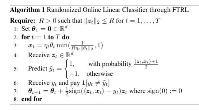
Putting all together, for example, we can have the following strategy using FTRL with regularizers 
Theorem 1 Let
an arbitrary sequence of samples/labels couples where
and
. Assume
, for
where
, for any
we have the following guarantee
![\displaystyle \mathop{\mathbb E}\left[\sum_{t=1}^T \boldsymbol{1}[\tilde{y}(\langle{\boldsymbol z}_t,{\boldsymbol x}_t\rangle) \neq y_t]\right] - \mathop{\mathbb E}\left[\sum_{t=1}^T \boldsymbol{1}[\tilde{y}(\langle{\boldsymbol z}_t,{\boldsymbol u}\rangle) \neq y_t] \right] \leq \sqrt{2 T}~.](https://s0.wp.com/latex.php?latex=%5Cdisplaystyle+%5Cmathop%7B%5Cmathbb+E%7D%5Cleft%5B%5Csum_%7Bt%3D1%7D%5ET+%5Cboldsymbol%7B1%7D%5B%5Ctilde%7By%7D%28%5Clangle%7B%5Cboldsymbol+z%7D_t%2C%7B%5Cboldsymbol+x%7D_t%5Crangle%29+%5Cneq+y_t%5D%5Cright%5D+-+%5Cmathop%7B%5Cmathbb+E%7D%5Cleft%5B%5Csum_%7Bt%3D1%7D%5ET+%5Cboldsymbol%7B1%7D%5B%5Ctilde%7By%7D%28%5Clangle%7B%5Cboldsymbol+z%7D_t%2C%7B%5Cboldsymbol+u%7D%5Crangle%29+%5Cneq+y_t%5D+%5Cright%5D+%5Cleq+%5Csqrt%7B2+T%7D%7E.+&bg=ffffff&fg=000000&s=0&c=20201002)
Proof: The proof is straightforward from the FTRL regret bound with the chosen increasing regularizer.

2. The Perceptron Algorithm
The above strategy has the shortcoming of restricting the feasible vectors in a possibly very small set. In turn, this could make the performance of the competitor low. In turn, the performance of the online algorithm is only close to the one of the competitor.
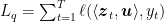
Another way to deal with the non-convexity is to compare the number of mistakes that the algorithm does with a convex cumulative loss of the competitor. That is, we can try to prove a weaker regret guarantee:
![\displaystyle \label{eq:weak_regret} \sum_{t=1}^T \boldsymbol{1}[y_t \neq \tilde{y}_t] - \sum_{t=1}^T \ell(\langle {\boldsymbol z}_t, {\boldsymbol u}\rangle, y_t) = O\left(\sqrt{T}\right)~. \ \ \ \ \ (1)](https://s0.wp.com/latex.php?latex=%5Cdisplaystyle+%5Clabel%7Beq%3Aweak_regret%7D+%5Csum_%7Bt%3D1%7D%5ET+%5Cboldsymbol%7B1%7D%5By_t+%5Cneq+%5Ctilde%7By%7D_t%5D+-+%5Csum_%7Bt%3D1%7D%5ET+%5Cell%28%5Clangle+%7B%5Cboldsymbol+z%7D_t%2C+%7B%5Cboldsymbol+u%7D%5Crangle%2C+y_t%29+%3D+O%5Cleft%28%5Csqrt%7BT%7D%5Cright%29%7E.+%5C+%5C+%5C+%5C+%5C+%281%29&bg=ffffff&fg=000000&s=0&c=20201002)
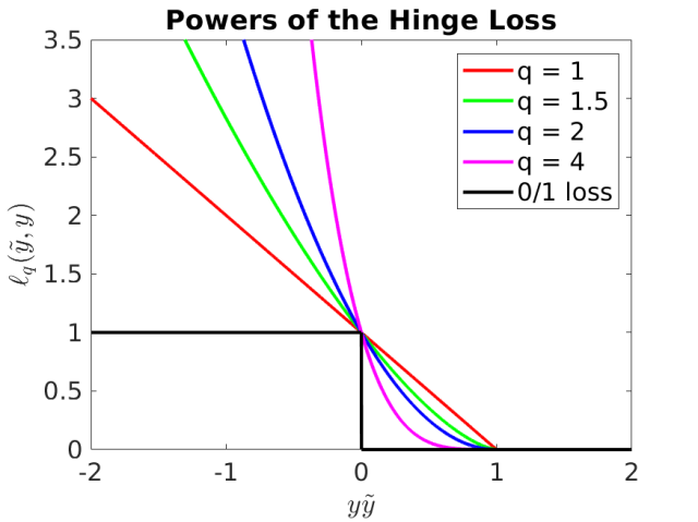
In particular, the convex loss we consider is powers of the Hinge Loss: 
The oldest algorithm we have to minimize the modified regret in (1) is the Perceptron algorithm, in Algorithm 2.
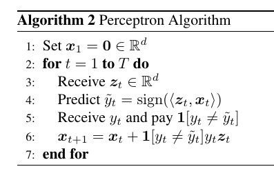
The Perceptron algorithm updates the current prediction 


In the same way, if 
For the Perceptron algorithm, we can prove the following guarantee.
Theorem 2 Let
![\displaystyle \sum_{t=1}^T \boldsymbol{1}[y_t \neq \tilde{y}_t] - \sum_{t=1}^T \ell(\langle {\boldsymbol z}_t, {\boldsymbol u}\rangle, y_t) \leq \frac{q^2 R^2 \|{\boldsymbol u}\|^2_2}{2} + q\|{\boldsymbol u}\|\sqrt{\frac{q^2 R^2 \|{\boldsymbol u}\|^2_2}{4} + \sum_{t=1}^T \ell_q(\langle {\boldsymbol z}_t, {\boldsymbol u}\rangle, y_t)},\ \forall {\boldsymbol u} \in {\mathbb R}^d, q\geq 1~.](https://s0.wp.com/latex.php?latex=%5Cdisplaystyle+%5Csum_%7Bt%3D1%7D%5ET+%5Cboldsymbol%7B1%7D%5By_t+%5Cneq+%5Ctilde%7By%7D_t%5D+-+%5Csum_%7Bt%3D1%7D%5ET+%5Cell%28%5Clangle+%7B%5Cboldsymbol+z%7D_t%2C+%7B%5Cboldsymbol+u%7D%5Crangle%2C+y_t%29+%5Cleq+%5Cfrac%7Bq%5E2+R%5E2+%5C%7C%7B%5Cboldsymbol+u%7D%5C%7C%5E2_2%7D%7B2%7D+%2B+q%5C%7C%7B%5Cboldsymbol+u%7D%5C%7C%5Csqrt%7B%5Cfrac%7Bq%5E2+R%5E2+%5C%7C%7B%5Cboldsymbol+u%7D%5C%7C%5E2_2%7D%7B4%7D+%2B+%5Csum_%7Bt%3D1%7D%5ET+%5Cell_q%28%5Clangle+%7B%5Cboldsymbol+z%7D_t%2C+%7B%5Cboldsymbol+u%7D%5Crangle%2C+y_t%29%7D%2C%5C+%5Cforall+%7B%5Cboldsymbol+u%7D+%5Cin+%7B%5Cmathbb+R%7D%5Ed%2C+q%5Cgeq+1%7E.+&bg=ffffff&fg=000000&s=0&c=20201002)
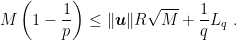
Before proving the theorem, let’s take a look to its meaning. If there exists a 


Remember that a hyperplane represented by its normal vector 


Also, given that we are considering a 

If the problem is not linearly separable, the Perceptron algorithm satisfies a regret of 

- The Perceptron is independent of scaling of the update by a hypothetical learning rate
, in the sense that the mistakes it does are independent of the scaling. That is, we could update with
and have the same mistakes and updates because they only depend on the sign of
. Hence, we can think as it is always using the best possible learning rate
- The weakened definition of regret allows to consider a family of loss functions, because the Perceptron is not using any of them in the update.
Let’s now prove the regret guarantee. For the proof, we will need the two following technical lemmas.
Lemma 3 (F. Cucker and D. X. Zhou, 2007, Lemma 10.17) Let
be such that
. Then

 ,
,  , and
, and  such that
  . Then,
  .
. Proof: Let 


Proof: } Denote by the total number of the mistakes of the Perceptron algorithm by ![{M=\sum_{t=1}^T \boldsymbol{1}[y_t \neq \tilde{y}_t]}](https://s0.wp.com/latex.php?latex=%7BM%3D%5Csum_%7Bt%3D1%7D%5ET+%5Cboldsymbol%7B1%7D%5By_t+%5Cneq+%5Ctilde%7By%7D_t%5D%7D&bg=ffffff&fg=000000&s=0&c=20201002)
First, note that the Perceptron algorithm can be thought as running Online Subgradient Descent (OSD) with a fixed stepsize ![{\tilde{\ell}_t({\boldsymbol x})=-\langle \boldsymbol{1}[y_t\neq \tilde{y}_t] y_t {\boldsymbol z}_t, {\boldsymbol x}\rangle}](https://s0.wp.com/latex.php?latex=%7B%5Ctilde%7B%5Cell%7D_t%28%7B%5Cboldsymbol+x%7D%29%3D-%5Clangle+%5Cboldsymbol%7B1%7D%5By_t%5Cneq+%5Ctilde%7By%7D_t%5D+y_t+%7B%5Cboldsymbol+z%7D_t%2C+%7B%5Cboldsymbol+x%7D%5Crangle%7D&bg=ffffff&fg=000000&s=0&c=20201002)

![\displaystyle \label{eq:proof_perc_eq1} {\boldsymbol x}_{t+1}={\boldsymbol x}_t + \eta\boldsymbol{1}[y_t\neq \tilde{y}_t] y_t{\boldsymbol z}_t~. \ \ \ \ \ (2)](https://s0.wp.com/latex.php?latex=%5Cdisplaystyle+%5Clabel%7Beq%3Aproof_perc_eq1%7D+%7B%5Cboldsymbol+x%7D_%7Bt%2B1%7D%3D%7B%5Cboldsymbol+x%7D_t+%2B+%5Ceta%5Cboldsymbol%7B1%7D%5By_t%5Cneq+%5Ctilde%7By%7D_t%5D+y_t%7B%5Cboldsymbol+z%7D_t%7E.+%5C+%5C+%5C+%5C+%5C+%282%29&bg=ffffff&fg=000000&s=0&c=20201002)
Now, as said above,
![\displaystyle \sum_{t=1}^T -\langle \boldsymbol{1}[y_t\neq \tilde{y}_t] y_t {\boldsymbol z}_t, {\boldsymbol x}_t\rangle + \sum_{t=1}^T \langle \boldsymbol{1}[y_t\neq \tilde{y}_t] y_t {\boldsymbol z}_t, {\boldsymbol u}\rangle \leq \frac{\|{\boldsymbol u}\|^2}{2\eta} + \frac{\eta}{2} \sum_{t=1}^T \boldsymbol{1}[y_t\neq \tilde{y}_t] \|{\boldsymbol z}_t\|^2_2, \ \forall \eta>0~.](https://s0.wp.com/latex.php?latex=%5Cdisplaystyle+%5Csum_%7Bt%3D1%7D%5ET+-%5Clangle+%5Cboldsymbol%7B1%7D%5By_t%5Cneq+%5Ctilde%7By%7D_t%5D+y_t+%7B%5Cboldsymbol+z%7D_t%2C+%7B%5Cboldsymbol+x%7D_t%5Crangle+%2B+%5Csum_%7Bt%3D1%7D%5ET+%5Clangle+%5Cboldsymbol%7B1%7D%5By_t%5Cneq+%5Ctilde%7By%7D_t%5D+y_t+%7B%5Cboldsymbol+z%7D_t%2C+%7B%5Cboldsymbol+u%7D%5Crangle+%5Cleq+%5Cfrac%7B%5C%7C%7B%5Cboldsymbol+u%7D%5C%7C%5E2%7D%7B2%5Ceta%7D+%2B+%5Cfrac%7B%5Ceta%7D%7B2%7D+%5Csum_%7Bt%3D1%7D%5ET+%5Cboldsymbol%7B1%7D%5By_t%5Cneq+%5Ctilde%7By%7D_t%5D+%5C%7C%7B%5Cboldsymbol+z%7D_t%5C%7C%5E2_2%2C+%5C+%5Cforall+%5Ceta%3E0%7E.+&bg=ffffff&fg=000000&s=0&c=20201002)
Given that this inequality holds for any
![\displaystyle \label{eq:proof_perc_eq2} \sum_{t=1}^T -\langle \boldsymbol{1}[y_t\neq \tilde{y}_t] y_t {\boldsymbol z}_t, {\boldsymbol x}_t\rangle + \sum_{t=1}^T \langle \boldsymbol{1}[y_t\neq \tilde{y}_t] y_t {\boldsymbol z}_t, {\boldsymbol u}\rangle \leq \|{\boldsymbol u}\| \sqrt{\sum_{t=1}^T \boldsymbol{1}[y_t\neq \tilde{y}_t] \|{\boldsymbol z}_t\|^2_2} \leq \|{\boldsymbol u}\| R\sqrt{\sum_{t=1}^T \boldsymbol{1}[y_t\neq \tilde{y}_t]}~. \ \ \ \ \ (3)](https://s0.wp.com/latex.php?latex=%5Cdisplaystyle+%5Clabel%7Beq%3Aproof_perc_eq2%7D+%5Csum_%7Bt%3D1%7D%5ET+-%5Clangle+%5Cboldsymbol%7B1%7D%5By_t%5Cneq+%5Ctilde%7By%7D_t%5D+y_t+%7B%5Cboldsymbol+z%7D_t%2C+%7B%5Cboldsymbol+x%7D_t%5Crangle+%2B+%5Csum_%7Bt%3D1%7D%5ET+%5Clangle+%5Cboldsymbol%7B1%7D%5By_t%5Cneq+%5Ctilde%7By%7D_t%5D+y_t+%7B%5Cboldsymbol+z%7D_t%2C+%7B%5Cboldsymbol+u%7D%5Crangle+%5Cleq+%5C%7C%7B%5Cboldsymbol+u%7D%5C%7C+%5Csqrt%7B%5Csum_%7Bt%3D1%7D%5ET+%5Cboldsymbol%7B1%7D%5By_t%5Cneq+%5Ctilde%7By%7D_t%5D+%5C%7C%7B%5Cboldsymbol+z%7D_t%5C%7C%5E2_2%7D+%5Cleq+%5C%7C%7B%5Cboldsymbol+u%7D%5C%7C+R%5Csqrt%7B%5Csum_%7Bt%3D1%7D%5ET+%5Cboldsymbol%7B1%7D%5By_t%5Cneq+%5Ctilde%7By%7D_t%5D%7D%7E.+%5C+%5C+%5C+%5C+%5C+%283%29&bg=ffffff&fg=000000&s=0&c=20201002)
Note that ![{-\boldsymbol{1}[y_t\neq \tilde{y}_t]y_t\langle {\boldsymbol z}_t, {\boldsymbol x}_t\rangle\geq 0}](https://s0.wp.com/latex.php?latex=%7B-%5Cboldsymbol%7B1%7D%5By_t%5Cneq+%5Ctilde%7By%7D_t%5Dy_t%5Clangle+%7B%5Cboldsymbol+z%7D_t%2C+%7B%5Cboldsymbol+x%7D_t%5Crangle%5Cgeq+0%7D&bg=ffffff&fg=000000&s=0&c=20201002)

So, denoting by ![{\tau_t=\boldsymbol{1}[y_t\neq \tilde{y}_t]}](https://s0.wp.com/latex.php?latex=%7B%5Ctau_t%3D%5Cboldsymbol%7B1%7D%5By_t%5Cneq+%5Ctilde%7By%7D_t%5D%7D&bg=ffffff&fg=000000&s=0&c=20201002)

where we used Holder’s inequality and
Given that 

Let’s now consider two cases. For 


that implies
Using the fact that 
Finally, using Lemma 4, we have the stated bound.
3. History Bits
The Perceptron was proposed by Rosenblatt (F. Rosenblatt, 1958). The proof of convergence in the non-separable case for 

Hi Francesco, in Algorithm 1 line 3 when we do the projection shouldn’t R be in the denominator?
Nicolò
LikeLike
Hi Nicolò, no, this looks correct to me: the first term in the min is selected when the norm is bigger than R, and projected back to R, no?
LikeLike
But didn’t we assume the norm of x bounded by 1 / R ? you say “choose the feasible set {V=\{{\boldsymbol x} \in{\mathbb R}^d : \|{\boldsymbol x}\|\leq \frac{1}{R}\}}. “
LikeLiked by 1 person
You are right! Fixed, thanks!
LikeLike