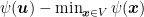
This post is part of the lecture notes of my class “Introduction to Online Learning” at Boston University, Fall 2019.
You can find all the lectures I published here.
Today, we will see a couple of practical implementations of online mirror descent, with two different Bregman functions and we will introduce the setting of Learning with Expert Advice.
1. Exponentiated Gradient
Let 


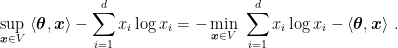
The Fenchel conjugate 

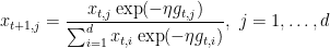
The solution is 
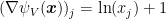
We also have 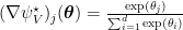
Putting all together, we have the online mirror descent update rule for entropic distance generating function.

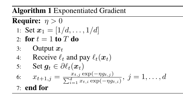
The algorithm is summarized in Algorithm 1. This algorithm is called Exponentiated Gradient (EG) because in the update rule we take the component-wise exponent of the gradient vector.
Let’s take a look at the regret bound we get. First, as we said, observe that

that is the KL divergence between the 1-dimensional discrete distributions 


Lemma 1 (S. Shalev-Shwartz, 2007, Lemma 16)
is 1-strongly convex with respect to the
norm over the set
.
Another thing to decide is the initial point 


![{{\boldsymbol x}_1=[1/d, \dots, 1/d] \in {\mathbb R}^d}](https://s0.wp.com/latex.php?latex=%7B%7B%5Cboldsymbol+x%7D_1%3D%5B1%2Fd%2C+%5Cdots%2C+1%2Fd%5D+%5Cin+%7B%5Cmathbb+R%7D%5Ed%7D&bg=ffffff&fg=000000&s=0&c=20201002)

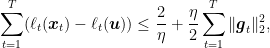
Putting all together, we have

Assuming 


Remark 1 Note that the time-varying version of OMD with entropic distance generating function would give rise to a vacuous bound, can you see why? We will see how FTRL overcomes this issue using a time-varying regularizer rather than a time-varying learning rate.
How would Online Subgradient Descent (OSD) work on the same problem? First, it is important to realize that nothing prevents us to use OSD on this problem. We just have to implement the euclidean projection onto the simplex. The regret bound we would get from OSD is
for any 


So, as we already saw analyzing AdaGrad, the shape of the domain is the important ingredient when we change from euclidean norms to other norms.
2. 
Consider the distance generating function 


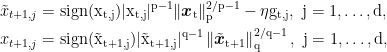
where we broke the update in two steps to simplify the notation (and the implementation). Starting from 

The last ingredient is the fact that 


Lemma 2 (S. Shalev-Shwartz, 2007, Lemma 17)
-strongly convex with respect to
.
Hence, the regret bound will be

Setting 

Also, note that 

Setting 

Assuming 


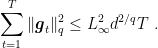
Note that 

So, the 
3. Learning with Expert Advice
Let’s introduce a particular Online Convex Optimization game called Learning with Expert Advice.
In this setting, we have
Is this problem solvable? If we put ourselves in the adversarial setting, unfortunately it cannot be solved! Indeed, even with 2 experts, the adversary can force on us linear regret. Let’s see how. In each round we have to pick expert 1 or expert 2. In each round, the adversary can decide that the expert we pick has loss 1 and the other one has loss 0. This means that the cumulative loss of the algorithm over 

The problem above is due to the fact that the adversary has too much power. One way to reduce its power is using randomization. We can allow the algorithm to be randomized and force the adversary to decide the losses at time 
First, let’s write the problem in the original formulation. We set a discrete feasible set 


The only thing that makes this problem non-convex is the feasibility set, that is clearly a non-convex one.
Let’s now see how the randomization makes this problem convex. Let’s extend the feasible set to 

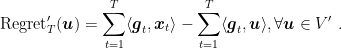
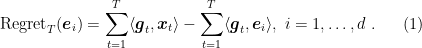
Can we find a way to transform an upper bound to this regret to the one we care in (1)? One way is the following one: On each time step, construct a random variable 


![\displaystyle \mathop{\mathbb E}[g_{t,i_t}] = \langle {\boldsymbol g}_t,{\boldsymbol x}_t\rangle,](https://s0.wp.com/latex.php?latex=%5Cdisplaystyle+%5Cmathop%7B%5Cmathbb+E%7D%5Bg_%7Bt%2Ci_t%7D%5D+%3D+%5Clangle+%7B%5Cboldsymbol+g%7D_t%2C%7B%5Cboldsymbol+x%7D_t%5Crangle%2C+&bg=ffffff&fg=000000&s=0&c=20201002)
and
![\displaystyle \mathop{\mathbb E}[\text{Regret}_T({\boldsymbol e}_i)] = \mathop{\mathbb E}[\text{Regret}'_T({\boldsymbol e}_i)] = \mathop{\mathbb E}\left[\sum_{t=1}^T \langle {\boldsymbol g}_{t}, {\boldsymbol x}_t\rangle - \sum_{t=1}^T \langle {\boldsymbol g}_t, {\boldsymbol e}_i\rangle\right]~.](https://s0.wp.com/latex.php?latex=%5Cdisplaystyle+%5Cmathop%7B%5Cmathbb+E%7D%5B%5Ctext%7BRegret%7D_T%28%7B%5Cboldsymbol+e%7D_i%29%5D+%3D+%5Cmathop%7B%5Cmathbb+E%7D%5B%5Ctext%7BRegret%7D%27_T%28%7B%5Cboldsymbol+e%7D_i%29%5D+%3D+%5Cmathop%7B%5Cmathbb+E%7D%5Cleft%5B%5Csum_%7Bt%3D1%7D%5ET+%5Clangle+%7B%5Cboldsymbol+g%7D_%7Bt%7D%2C+%7B%5Cboldsymbol+x%7D_t%5Crangle+-+%5Csum_%7Bt%3D1%7D%5ET+%5Clangle+%7B%5Cboldsymbol+g%7D_t%2C+%7B%5Cboldsymbol+e%7D_i%5Crangle%5Cright%5D%7E.+&bg=ffffff&fg=000000&s=0&c=20201002)
This means that we can minimize in expectation the non-convex regret with a randomized OCO algorithm. We can summarize this reasoning in Algorithm 2.

For example, if we use EG as the OCO algorithm, setting ![{{\boldsymbol x}_1=[1/d, \dots, 1/d]}](https://s0.wp.com/latex.php?latex=%7B%7B%5Cboldsymbol+x%7D_1%3D%5B1%2Fd%2C+%5Cdots%2C+1%2Fd%5D%7D&bg=ffffff&fg=000000&s=0&c=20201002)
and the regret will be
![\displaystyle \mathop{\mathbb E}[\text{Regret}_T({\boldsymbol e}_i)] \leq \frac{\sqrt{2}}{2} L_\infty \sqrt{T \ln d}, \ \forall {\boldsymbol e}_i~.](https://s0.wp.com/latex.php?latex=%5Cdisplaystyle+%5Cmathop%7B%5Cmathbb+E%7D%5B%5Ctext%7BRegret%7D_T%28%7B%5Cboldsymbol+e%7D_i%29%5D+%5Cleq+%5Cfrac%7B%5Csqrt%7B2%7D%7D%7B2%7D+L_%5Cinfty+%5Csqrt%7BT+%5Cln+d%7D%2C+%5C+%5Cforall+%7B%5Cboldsymbol+e%7D_i%7E.+&bg=ffffff&fg=000000&s=0&c=20201002)
It is worth stressing the importance of the result just obtained: We can design an algorithm that in expectation is close to the best expert in a set, paying only a logarithmic penalty in the size of the set.
In the future, we will see algorithms that achieve even the better regret guarantee of 


4. History Bits
The EG algorithm was introduced by (Kivinen, J. and Warmuth, M., 1997), but not as a specific instantiation of OMD. I am actually not sure when people first pointed out the link between EG and OMD, do you know something about this? If yes, please let me know! Beck and Teboulle (2003) rediscover EG for the offline case as an example of Mirror Descent. Later, Cesa-Bianchi and Lugosi (2006) show that EG is just an instantiation of OMD.
The trick to set 
5. Exercises
Exercise 1 Derive the EG update rule and regret bound in the case that the algorithm starts from an arbitrary vector
6. Appendix
Here we find the conjugate of the negative entropy.
It is a constrained optimization problem, we can solve it using the KKT conditions. We first rewrite it as a minimization problem
The KKT conditions are, for 
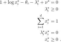
From the first one we get 


Denoting with 


Hi Francesco, nice post as always!
Two typos: when you define the set X in the beginning after the Exponentiated Gradient algorithm, it should be \| x \|_1 = 1. And then, when you discuss the suboptimality of OSD wrt EG the difference in the regret bound is \sqrt(d) vs \sqrt(ln d), not just ln d, right?
Also, I have few questions. Regarding remark 1, is the problem related to the fact that in the time-varying version of OMD the KL divergence between u and x_t could potentially explode for some t, if u_{i, t} is not 0 but x_{i, t} goes to 0 for some i?
The second is about p-norm algorithms. In the tuning of \eta, we introduce the parameter \alpha, because I guess we do not know \| u \|_1^2 and it shouldn’t matter on the order of the regret bound of O(\sqrt(T ln d)). However, how would you practically set it? This is indeed not parameter-free 😛
LikeLiked by 1 person
Thanks!
Typos fixed.
First question: yes. Probably that term is boundable in some way, but I suspect that you get something more that sqrt{T}. But I actually never tried.
Second question: I introduce alpha exactly to make you notice that there is an untuned parameter! In Online Learning papers you will find 3 different ways to cope with this problem: 1) assume to know ||u|| (that is impossible, given the adversarial nature of the game); 2) compete only with ||u||\leq U, where U is a parameter (bad idea: we still have a parameter and bound now depends on U); 3) say that the order of the bound is the same even if you don’t tune it (it assumes that argmin_u sum_{t=1}^T l_t(u) exists, but this is false in many settings, e.g. logistic regression on a separable dataset and regression with a universal kernel. I discussed the logistic case when explaining a variant of online-to-batch).
We will be able to remove the need of that parameter completely when we will use the coin-betting methods, I’ll add a link to this.
LikeLike
Thank you for the replies!
Regarding the first question, can’t we use a “clipped” simplex? I’m thinking of Fixed-Share kind of updates where we want to prevent weights going to 0 to force somehow additional exploration, thus we consider X = \{ x \in R^d: x_i \geq \alpha, \| x \|_1 = 1 \}. Then of course we should tune \alpha but maybe we can still get \sqrt{T}? (For the expert setting Fixed-Share kind of algorithms are \tilde{O}(\sqrt(T S \ln K)), where S is the number of shifts in the comparator sequence).
LikeLike
If you change V, then you have to explicitly compute the projection w.r.t. the Bregman divergence, that in this case is the KL divergence. I don’t know how difficult it would be.
A part from that, it might work, but I am not sure what is the advantage: FTRL gives use the right bound in this case, why using OMD? Also, even with your fix, you wouldn’t get the KL divergence between the first point and the competitor, but only the worst KL divergence in your “clipped” simplex.
LikeLike
Yes, I guess the FTRL solution is the best approach. I was just curious whether MD could be used with time-varying learning rates, since I don’t think I have seen such a case 🙂
LikeLike
Now that I think about it, David proved a lower bound in the journal version of our scale-free paper. It says that the regret of EG is linear in time if used with time-varying learning rates!
LikeLike
Cool! I’ll take a look at it, thanks 🙂
LikeLiked by 1 person
Thanks to Nicolò Cesa-Bianchi for answering to my question on the references on EG and OMD.
LikeLike
Hi Francesco,
Thanks for the post! When we’re comparing OSD and EG, regarding OSD, can we set x_1 = 0 which is actually infeasible?
LikeLike
You are right! I fixed it now
LikeLike