Online Gradient Descent

This post is part of the lecture notes of my class “Introduction to Online Learning” at Boston University, Fall 2019. I will publish two lectures per week.

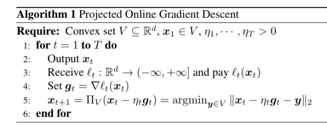
You can find the lectures I published till now here.

To summarize what we said in the previous note, let’s define online learning as the following general game

For
- Outputs ${{\boldsymbol x}_t \in V\subseteq {\mathbb R}^d}$
- Receive ${\ell_t:V \rightarrow {\mathbb R}}$
- Pay ${\ell_t({\boldsymbol x}_t)}$
End for

The aim of this game is to minimize the regret with respect to any competitor ${{\boldsymbol u} \in V}$ :

$\displaystyle \text{Regret}_T({\boldsymbol u}):=\sum_{t=1}^T \ell_t({\boldsymbol x}_t) - \sum_{t=1}^T \ell_t({\boldsymbol u})~.$

We also said that the way the losses ${\ell_t}$ are decided is adversarial. Now, without additional assumption we cannot hope to solve this problem. Hence, we have to understand what are the reasonable assumptions we can make. Typically, we will try to restrict the choice of the loss functions in some way. This is considered reasonable because most of the time we decide the set from which loss functions are picked. So, for example, we will consider only convex loss functions. However, convexity might not be enough, so we might restrict the class a bit more to, for example, Lipschitz convex functions. On the other hand, assuming to know something about the future is not considered a reasonable assumption, because we very rarely have any control on the future. In general, the stronger the assumptions the better will be the upper bound on the regret we can prove. The best algorithms we will see will guarantee a sublinear regret against the weakest assumption we can make, guaranteeing at the same time a smaller regret for easy adversaries.

It is also important to remember why minimizing the regret is a good objective: Given that we don’t assume anything on how the adversary generates the loss functions, minimizing the regret is a good metric that takes into account the difficulty of the problem. If an online learning algorithm is able to guarantee a sublinear regret, it means that its performance on average will approach the performance of any fixed strategy. As said, we will see that in many situations if the adversary is “weak”, for example it is a fixed stochastic distribution over the loss functions, being prepared for the worst-case scenario will not preclude us to get the best guarantee anyway.

For a while, we will focus on the case that ${\ell_t}$ are convex, and this problem will be called Online Convex Optimization (OCO). Later, we will later see how to convexify some non-convex online problems.

Why so much math?? I will now introduce some math concepts. If you have a background in Convex Analysis, this will be easy stuff for you. On the other hand, if you never saw these things before they might look a bit scary. Let me tell you the right way to look at them: these are tools that will make our job easier. Without these tools, it would be basically impossible to design any online learning algorithm. And, no, it is not enough to test random algorithms on some machine learning dataset, because fixed datasets are not adversarial. Without a correct proof, you might never realize that your online algorithm fail on particular sequences of losses, as it happened to Adam (Reddi, S. J. and Kale, S. and Kumar, S., 2018). I promise you that once you understand the key mathematical concepts, online learning is actually easy.

1. Convex Analysis Bits: Convexity

convex_nonconvex — Figure 1. Convex and non-convex sets.

Definition 1 ${V \subset {\mathbb R}^d}$ is convex if for any ${{\boldsymbol x},{\boldsymbol y}\in V}$ and any ${\lambda \in (0,1)}$ , we have

$\displaystyle \lambda {\boldsymbol x}+ (1-\lambda) {\boldsymbol y} \in V~.$

In words, this means that the set ${V}$ with no holes, see Figure 1.

We will make use of extended-real-valued functions, that is function that take value in ${{\mathbb R}\cup\{-\infty,+\infty\}}$ . For ${f}$ an extended-real-valued function on ${{\mathbb R}^d}$ , its domain is the set ${\mathop{\mathrm{dom}} f = \{{\boldsymbol x} \in {\mathbb R}^d : f(x) < +\infty\}}$ .

Extended-real-valued functions easily allow us to consider constrained set and are a standard notation in Convex Optimization, see, e.g., (Boyd, S. and Vandenberghe, L., 2004). For example, if I want the predictions of the algorithm ${x_t}$ and the competitor ${{\boldsymbol u}}$ to be in a set ${V \subset {\mathbb R}^d}$ , I can just add ${i_V({\boldsymbol x})}$ to all the losses, where ${i_V:{\mathbb R}^d\rightarrow (-\infty, +\infty]}$ is the indicator function of the set ${V}$ defined as

$\displaystyle i_V({\boldsymbol x}) = \begin{cases} 0, & {\boldsymbol x} \in V,\\ +\infty, & \text{otherwise.} \end{cases}$

In this way, the only way for the algorithm and for the competitor to suffer finite loss is to predict inside the set ${V}$ . Also, extended-real-valued functions will make the use of Fenchel conjugates more direct.

Figure 2. Convex and non-convex functions.

Convex functions will be an essential ingredient in online learning.

Definition 2 Let ${f:{\mathbb R}^d \rightarrow [-\infty, +\infty]}$ . ${f}$ is convex if the epigraph of the function, ${\{({\boldsymbol x}, y) \in {\mathbb R}^{d+1}| y\geq f(x)\}}$ , is convex.

We can see a visualization of this definition in Figure 2. Note that the definition implies that the domain of a convex function is convex. Also, observe that if ${f:V \subseteq {\mathbb R}^d \rightarrow {\mathbb R}}$ is convex, ${f + i_V: {\mathbb R}^d \rightarrow (-\infty, +\infty]}$ is convex.

Note that ${i_V({\boldsymbol x})}$ is convex iff ${V}$ is convex, so each convex set is associated with a convex function.

The definition above gives rise to the following characterization for convex functions that do not assume the value ${-\infty}$ .

Theorem 3 (Rockafellar, R. T., 1970, Theorem 4.1) Let ${f:{\mathbb R}^d\rightarrow (-\infty, +\infty]}$ and ${\mathop{\mathrm{dom}} f}$ is a convex set. Then ${f}$ is convex iff, for any ${0<\lambda <1}$ , we have

$\displaystyle f(\lambda {\boldsymbol x} + (1-\lambda) {\boldsymbol y}) \leq \lambda f({\boldsymbol x}) + (1-\lambda) f({\boldsymbol y}) \ \forall {\boldsymbol x}, {\boldsymbol y} \in \mathop{\mathrm{dom}} f~.$

Example 1 The simplest example of convex functions are the affine function: ${f({\boldsymbol x})=\langle {\boldsymbol z}, {\boldsymbol x}\rangle + b}$ .

Example 2 Norms are always convex, the proof is left as exercise.

How to recognize a convex function? In the most general case, you have to rely on the definition. However, most of the time we will recognize them as composed by operations that preserve the convexity. For example:

${f}$ and ${g}$ convex, then the linear combination with non-negative weights is also convex.
The composition with an affine transformation preserves the convexity.
Pointwise supremum of convex functions is convex.

The proofs are left as exercises.

A very important property of differentiable convex functions is that we can construct linear lower bound to the function.

Theorem 4 (Rockafellar, R. T., 1970, Theorem 25.1 and Corollary 25.1.1) Suppose ${f:{\mathbb R}^d\rightarrow (-\infty, +\infty]}$ a convex function and let ${{\boldsymbol x} \in \mathop{\mathrm{int}} \mathop{\mathrm{dom}} f}$ . If ${f}$ is differentiable at ${{\boldsymbol x}}$ then

$\displaystyle f({\boldsymbol y}) \geq f({\boldsymbol x}) + \langle \nabla f({\boldsymbol x}), {\boldsymbol y} - {\boldsymbol x}\rangle, \ {\boldsymbol y} \in {\mathbb R}^d~.$

We will also use the optimality condition for convex functions:

Theorem 5 Let ${V}$ a convex non-empty set, ${{\boldsymbol x}^\star \in V}$ , and ${f}$ a convex function, differentiable over an open set that contains ${V}$ . Then ${{\boldsymbol x}^\star = \mathop{\mathrm{argmin}}_{{\boldsymbol x} \in V} f({\boldsymbol x})}$ iff ${\langle \nabla f({\boldsymbol x}^\star), {\boldsymbol y} -{\boldsymbol x}^\star \rangle \geq 0, \ \forall {\boldsymbol y} \in V}$ .

In words, at the constrained minimum, the gradient makes an angle of ${90^\circ}$ or less with all the feasible variations ${{\boldsymbol y} - {\boldsymbol x}^\star}$ , hence we cannot minimize more the function moving inside ${V}$ .

Another critical property of convex functions is Jensen’s inequality.

Theorem 6 Let ${f : {\mathbb R}^d \rightarrow (-\infty, +\infty]}$ be a measurable convex function and ${{\boldsymbol x}}$ be an ${{\mathbb R}^d}$ -valued random element on some probability space such that ${\mathop{\mathbb E}[{\boldsymbol x}]}$ exists and ${{\boldsymbol x} \in \mathop{\mathrm{dom}} f}$ with probability 1. Then

$\displaystyle E[f({\boldsymbol x})] \geq f(E[{\boldsymbol x}])~.$

Let’s see our first OCO algorithm in the case that the functions are also differentable.

2. Online Gradient Descent

Last time we saw a simple strategy to obtain a logarithmic regret in the guessing game. The strategy was to use the best over the past, that is the Follow-the-Leader strategy. In formulas,

$\displaystyle {\boldsymbol x}_t=\mathop{\mathrm{argmin}}_{{\boldsymbol x}} \ \sum_{i=1}^{t-1} \ell_i({\boldsymbol x}),$

and in the first round we can play any admissible point. One might wonder if this strategy always works, but the answer is negative!

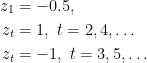
Example 3 (Failure of FTL) Let ${V = [-1,1]}$ and consider the sequence of losses ${\ell_t(x) = z_t x + i_V(x)}$ , where

$\displaystyle \begin{aligned} z_1 &= -0.5,\\ z_{t} &= 1, \ t=2, 4, \dots\\ z_{t} &= -1, \ t=3, 5, \dots \end{aligned}$

Then, a part from the first round where the prediction of FTL is arbitrary in ${[-1,1]}$ , the predictions of FTL will be ${x_t = 1}$ for ${t}$ even and ${x_t = -1}$ for ${t}$ odd. The cumulative loss of the FTL algorithm will therefore be ${T}$ while the cumulative loss of the fixed solution ${u = 0}$ is 0. Thus, the regret of FTL is ${T}$ .

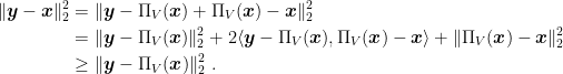
Hence, we will show an alternative strategy that guarantees sublinear regret for convex Lipschitz functions. Later, we will also prove that the dependency on ${T}$ is optimal. The strategy is called Projected Online Gradient Descent, or just Online Gradient Descent, see Algorithm 1. It consists in updating the prediction of the algorithm at each time step moving in the negative direction of the gradient of the loss received and projecting back onto the feasible set. It is similar to Stochastic Gradient Descent, but it is not the same thing: here the loss functions are different at each step. We will later see that Online Gradient Descent can also be used as Stochastic Gradient Descent.

pogd

First, we show the following two Lemmas. The first lemma proves that Euclidean projections always decrease the distance with points inside the set.

Proposition 7 Let ${{\boldsymbol x} \in {\mathbb R}^d}$ and ${{\boldsymbol y} \in V}$ , where ${V \subset {\mathbb R}^d}$ is a non-empty closed convex set and define ${\Pi_V({\boldsymbol x}):=\mathop{\mathrm{argmin}}_{{\boldsymbol y} \in V} \ \|{\boldsymbol x}-{\boldsymbol y}\|_2}$ . Then, ${\|\Pi_V({\boldsymbol x})-{\boldsymbol y}\|_2 \leq \|{\boldsymbol x}-{\boldsymbol y}\|_2}$ .

Proof: From the optimality condition of Theorem 5, we obtain

$\displaystyle \langle \Pi_V({\boldsymbol x})-{\boldsymbol x}, {\boldsymbol y}-\Pi_V({\boldsymbol x})\rangle \geq 0~.$

Therefore,

$\displaystyle \begin{aligned} \|{\boldsymbol y} - {\boldsymbol x}\|_2^2 &= \|{\boldsymbol y}-\Pi_V({\boldsymbol x})+\Pi_V({\boldsymbol x})-{\boldsymbol x}\|_2^2 \\ &= \|{\boldsymbol y}-\Pi_V({\boldsymbol x})\|^2_2 +2 \langle {\boldsymbol y}-\Pi_V({\boldsymbol x}),\Pi_V({\boldsymbol x})-{\boldsymbol x}\rangle + \|\Pi_V({\boldsymbol x})-{\boldsymbol x}\|_2^2 \\ &\geq \|{\boldsymbol y}-\Pi_V({\boldsymbol x})\|_2^2~. \end{aligned}$

$\Box$

The next lemma upper bounds the regret in one iteration of the algorithm.

Lemma 8 Let ${V\subset {\mathbb R}^d}$ a closed non-empty convex set and ${\ell_t:{\mathbb R}^d \rightarrow (-\infty, +\infty]}$ a convex function differentiable in a open set that contains ${V}$ . Set ${{\boldsymbol g}_t = \nabla \ell_t({\boldsymbol x}_t)}$ . Then, ${\forall {\boldsymbol u} \in V}$ , the following inequality holds

$\displaystyle \eta_t (\ell_t({\boldsymbol x}_t)- \ell_t({\boldsymbol u}) ) \leq \eta_t \langle {\boldsymbol g}_t, {\boldsymbol x}_t -{\boldsymbol u}\rangle \leq \frac{1}{2}\|{\boldsymbol x}_t-{\boldsymbol u}\|^2_2 - \frac{1}{2}\|{\boldsymbol x}_{t+1}-{\boldsymbol u}\|^2_2 + \frac{\eta_t^2}{2}\|{\boldsymbol g}_t\|_2^2~.$

Proof: From Proposition 7 and Theorem 4, we have that

$\displaystyle \begin{aligned} \|{\boldsymbol x}_{t+1}-{\boldsymbol u}\|^2_2 - \|{\boldsymbol x}_{t}-{\boldsymbol u}\|^2_2 &\leq \|{\boldsymbol x}_t-\eta_t {\boldsymbol g}_t -{\boldsymbol u}\|^2_2 - \|{\boldsymbol x}_{t}-{\boldsymbol u}\|^2_2 \\ &= -2 \eta_t \langle {\boldsymbol g}_t, {\boldsymbol x}_t - {\boldsymbol u}\rangle + \eta_t^2 \|{\boldsymbol g}_t\|^2_2 \\ &\leq -2 \eta_t (\ell_t({\boldsymbol x}_t) - \ell_t({\boldsymbol u})) + \eta_t^2 \|{\boldsymbol g}_t\|^2_2~. \end{aligned}$

Reordering, we have the stated bound. $\Box$

We can prove the following regret guarantee in the online setting.

Theorem 9 Let ${V\subseteq {\mathbb R}^d}$ a closed non-empty convex set with diameter ${D}$ , i.e. ${\max_{{\boldsymbol x},{\boldsymbol y}\in V} \|{\boldsymbol x}-{\boldsymbol y}\|_2 \leq D}$ . Let ${\ell_1, \cdots, \ell_T}$ an arbitrary sequence of convex functions ${\ell_t:{\mathbb R}^d \rightarrow (-\infty, +\infty]}$ differentiable in open sets containing ${V}$ for ${t=1, \dots,T}$ . Pick any ${{\boldsymbol x}_1 \in V}$ assume ${\eta_{t+1}\leq \eta_{t}, \ t=1, \dots, T}$ . Then, ${\forall {\boldsymbol u} \in V}$ , the following regret bound holds

$\displaystyle \sum_{t=1}^T (\ell_t({\boldsymbol x}_t) - \ell_t({\boldsymbol u})) \leq \frac{D^2}{2\eta_{T}} + \sum_{t=1}^T \frac{\eta_t}{2} \|{\boldsymbol g}_t\|^2_2~.$

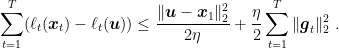
Moreover, if ${\eta_t}$ is constant, i.e. ${\eta_t=\eta \ \forall t=1,\cdots,T}$ , we have

$\displaystyle \sum_{t=1}^T (\ell_t({\boldsymbol x}_t) - \ell_t({\boldsymbol u})) \leq \frac{\|{\boldsymbol u}-{\boldsymbol x}_1\|_2^2}{2\eta} + \frac{\eta}{2} \sum_{t=1}^T \|{\boldsymbol g}_t\|^2_2~.$

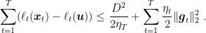
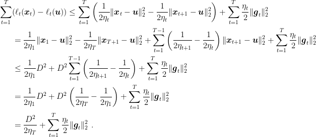
Proof: Dividing the inequality in Lemma 8 by ${\eta_t}$ and summing over ${t=1,\cdots,T}$ , we have

$\displaystyle \begin{aligned} \sum_{t=1}^T &(\ell_t({\boldsymbol x}_t) - \ell_t({\boldsymbol u})) \leq \sum_{t=1}^T \left(\frac{1}{2\eta_t}\|{\boldsymbol x}_{t}-{\boldsymbol u}\|^2_2 - \frac{1}{2\eta_t}\|{\boldsymbol x}_{t+1}-{\boldsymbol u}\|^2_2\right) + \sum_{t=1}^T \frac{\eta_t}{2} \|{\boldsymbol g}_t\|^2_2 \\ &= \frac{1}{2\eta_1}\|{\boldsymbol x}_{1}-{\boldsymbol u}\|^2_2 - \frac{1}{2\eta_T} \|{\boldsymbol x}_{T+1}-{\boldsymbol u}\|^2_2 + \sum_{t=1}^{T-1} \left(\frac{1}{2\eta_{t+1}}-\frac{1}{2\eta_t}\right)\|{\boldsymbol x}_{t+1}-{\boldsymbol u}\|^2_2 + \sum_{t=1}^T \frac{\eta_t}{2} \|{\boldsymbol g}_t\|^2_2 \\ &\leq \frac{1}{2\eta_1} D^2 + D^2 \sum_{t=1}^{T-1} \left(\frac{1}{2\eta_{t+1}}-\frac{1}{2\eta_{t}}\right) + \sum_{t=1}^T \frac{\eta_t}{2} \|{\boldsymbol g}_t\|^2_2 \\ &= \frac{1}{2\eta_1} D^2 + D^2 \left(\frac{1}{2\eta_{T}}-\frac{1}{2\eta_1}\right) + \sum_{t=1}^T \frac{\eta_t}{2} \|{\boldsymbol g}_t\|^2_2 \\ &= \frac{D^2}{2\eta_{T}} + \sum_{t=1}^T \frac{\eta_t}{2} \|{\boldsymbol g}_t\|^2_2~. \end{aligned}$

The proof of the second statement is left as an exercise. $\Box$

We can immediately observe few things.

If we want to use time-varying learning rates you need a bounded domain ${V}$ . However, this assumption is false in most of the machine learning applications. However, in the stochastic setting you can still use a time-varying learning rate in SGD with an unbounded domain if you use a non-uniform averaging. We will see this later.
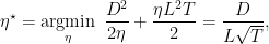
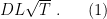
Another important observation is that the regret bound helps us choosing the learning rates ${\eta_t}$ . Indeed, it is the only guideline we have. Any other choice that is not justified by a regret analysis it is not justified at all.

As we said, the presence of parameters like the learning rates make no sense in online learning. So, we have to decide a strategy to set them. A simple choice is to find the constant learning rate that minimizes the bounds for a fixed number of iterations. We have to consider the expression

$\displaystyle \frac{\|{\boldsymbol u}-{\boldsymbol x}_1\|_2^2}{2\eta} + \frac{\eta}{2} \sum_{t=1}^T \|{\boldsymbol g}_t\|_2^2$

and minimize with respect to ${\eta}$ . It is easy to see that the optimal ${\eta}$ is ${\frac{\|{\boldsymbol u}-{\boldsymbol x}_1\|}{\sqrt{\sum_{t=1}^T \|{\boldsymbol g}_t\|_2^2}}}$ , that would give the regret bound

$\displaystyle \|{\boldsymbol u}-{\boldsymbol x}_1\|_2\sqrt{\sum_{t=1}^T \|{\boldsymbol g}_t\|_2^2}~.$

However, we have a problem: in order to use this stepsize, we should know all the future subgradients and the distance between the optimal solution and the initial point! This is clearly impossible: Remember that the adversary can choose the sequence of functions. Hence, it can observe your choice of learning rates and decide the sequence so that your learning rate is now the wrong one!

Indeed, it turns out that this kind of rate is completely impossible because it is ruled out by a lower bound. Yet, we will see that it is indeed possible to achieve very similar rates using adaptive and parameter-free algorithms.

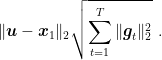
In the following, we will see many adaptive strategies. For the moment, we can observe that we might be happy to minimize a looser upper bound. In particular, assume that the norm of the gradients is bounded by ${L}$ , that is ${\|{\boldsymbol g}_t\|_2 \leq L}$ . Also, assuming a bounded diameter, we can upper bound ${\|{\boldsymbol u}-{\boldsymbol x}_1\|}$ by ${D}$ . Hence, we have

$\displaystyle \eta^\star = \mathop{\mathrm{argmin}}_\eta \ \frac{D^2}{2\eta} + \frac{\eta L^2 T}{2} = \frac{D}{L \sqrt{T}},$

that gives a regret bound of

$\displaystyle \label{eq:pogd_tuned_regret} D L \sqrt{T}~. \ \ \ \ \ (1)$

So, indeed the regret is sublinear in time. Next time, we will see how to remove the differentiability assumption through the use of subgradients.

3. History Bits

The Projected Online Subgradient Descent with time-varying learning rate and the concept itself of Online Convex Optimization was introduced by (M. Zinkevich, 2003). Note that, if we consider the optimization literature, the optimization people never restricted themselves to the bounded case.

4. Exercises

Exercise 1 Prove the second part of Theorem 9.

Exercise 2 Prove that ${\sum_{t=1}^T \frac{1}{\sqrt{t}} \leq 2\sqrt{T}-1}$ .

Exercise 3 Using the inequality in the previous exercise, prove that a learning rate ${\eta_t\propto \frac{1}{\sqrt{t}}}$ gives rise to a regret only a constant multiplicative factor worse than the one in (1).

14 Comments

Pingback: More Online-to-Batch Examples and Strong Convexity – Parameter-free Learning and Optimization Algorithms
Pingback: Lower Bounds for Online Linear Optimization – Parameter-free Learning and Optimization Algorithms
Pingback: Follow-The-Regularized-Leader I: Regret Equality – Parameter-free Learning and Optimization Algorithms
Pingback: Subgradients and Online-to-Batch conversion – Parameter-free Learning and Optimization Algorithms
LCella says:

December 7, 2019 at 10:14 AM

Hi,
Am I wrong or in the first line of the Proof of Theorem 9, the second inequality of Lemma 8 has to be divided by \eta_t instead of 2 \eta_t ?

Besides this minor detail, I was wondering if the choice of the adaptive parameter in Exercise 3 is taken by “converting to online” the ideal batch choice \eta= $\frac{D}{LT}$.

Thanks

LikeLike

1. bremen79 says:
  
  December 7, 2019 at 10:39 AM
  
  Typo fixed, thanks!
  The choice of the time-varying learning rate in Exercise 3 does indeed corresponds to make the choice eta proportional 1/sqrt{T} to an “online version” of eta_t proportional to 1/sqrt{t}. However, the reason why it works seems to be purely mathematical. In other words, it is not true that any fixed choice of parameters can be made “online” in a natural way: Each time you’ll have to prove that it works by proving the regret guarantee.
  
  LikeLike
  
Pingback: Last Iterate of SGD Converges (Even in Unbounded Domains) – Parameter-free Learning and Optimization Algorithms
Pingback: Neural Network (Maybe) Evolved to Make Adam The Best Optimizer – Parameter-free Learning and Optimization Algorithms
Pingback: Perceptron is Not SGD: A Better Interpretation Through Pseudogradients – Parameter-free Learning and Optimization Algorithms
Pingback: Saddle-Point Problems and OCO – Parameter-free Learning and Optimization Algorithms
Jacopo Molinari says:

December 16, 2021 at 4:59 AM

Hi,
I’m in trouble with the beginning of the Proof of Proposition 7; how can you obtain the vectors of the inner product from the Optimality condition of Theorem 5?
Pheraps it is just a gap of mine in algebra. Anyway, I tried to find a way to “connect” the things but I wasn’t able to.
Could you please explain me how to?

Thanks

LikeLike

1. bremen79 says:
  
  December 16, 2021 at 5:09 AM
  
  Hi Jacopo, there are a couple of skipped steps: we want to apply the optimality condition of the objective function of the projection. Now, instead of doing it directly, we first observe that the argmin of the projection does not change if instead of considering ||x-y||, we consider 1/2 ||x-y||^2. Taking the gradient of this function and using the optimality condition should give you the inner product. Can you see it now?
  
  LikeLike
  
Wood says:

September 14, 2022 at 5:16 AM

Hi
I am in trouble to understand Lemma 2.12. Why Lt(Xt) – Lt(u) <= ? From Theorem 2.7, we can get Lt(Xt) >= Lt(u) + . Could you pls give me more explain?

Thanks

LikeLike

bremen79 says:

September 14, 2022 at 9:47 AM

In theorem 2.7 set x=x_t and y=u, to obtain f(u) >= f(x_t) + inner product. Now, just reorder the terms and bring the negative sign inside the inner product.

LikeLike

wisdom says:

April 6, 2023 at 10:35 AM

In proof of theorem 9: do we know any relation between $$n_t$$’s ?
like that n1>n2>… and so on? (the learning rate)

LikeLike

1. bremen79 says:
  
  April 6, 2023 at 11:20 AM
  
  As stated in the assumptions of the theorem, for the first bound we assume the learning rate to be non-increasing. So, it can stay constant or decrease between one iteration and the following one.
  
  LikeLiked by 1 person
  
Pingback: Proof of online gradient descent regret bound – Mathematics – Forum
Pingback: Adapting to Smoothness with Normalized Gradients – Parameter-free Learning and Optimization Algorithms
rpSebastian says:

September 10, 2023 at 12:12 PM

Hello

In Theorem 9, could you please explain the role of the assumption $\eta_{t+1} \le \eta_t$? It seems like this assumption is not directly utilized in the proof.

Thanks a lot.

LikeLike

1. bremen79 says:
  
  September 10, 2023 at 12:16 PM
  
  In the second inequality, you need 1/eta_{t+1}-1/eta_t to be positive to be able to upper bound ||x_{t+1}-u|| with D
  
  LikeLike
  
  1. rpSebastian says:
    
    September 10, 2023 at 10:32 PM
    
    Thank you for your guidance. I realized that I overlooked the point.
    
    I find that if we assume $\eta_{t+1} > \eta$, we can still obtain a similar regret bound. In this case, when the term $1/\eta_{t+1}-1/\eta_t$ is negative, we obtain the bound $1/(2\eta_1) ||x_1 – u||2^2 + \sum_{t=1}^{T} \eta_t/2 ||g_t||_2^2$.
    
    This assumption, $\eta_{t+1} > \eta_t$, seems to suggest that even with an increasing learning rate, the algorithm still converges. Is my understanding correct, or could this assumption have other effects on the algorithm?
    
    LikeLiked by 1 person
  2. bremen79 says:
    
    September 11, 2023 at 1:08 AM
    
    You are correct that even increasing learning rate gives you something. But to get sqrt(T) regret you still need the term sum_{t=1}^{T} eta_t/2 ||g_t||_2^2 to be of the order of sqrt{T}, so eta_t cannot grow too fast. There are papers on the learning with expert setting where they use a mildly increasing learning rate to take advantage of an additional negative term in the regret.
    
    LikeLike
  3. rpSebastian says:
    
    September 11, 2023 at 2:35 AM
    
    I will take a look at relevant papers. Thanks very much!
    
    LikeLiked by 1 person
Pingback: Is Nesterov’s Universal Algorithm Really Universal? – Parameter-free Learning and Optimization Algorithms
Yanze says:

February 4, 2024 at 5:18 PM

Hello! Thanks for the post!

Regarding OGD, I get that mathematically it’ll enjoy optimal regret under some conditions, which is good! But how do we understanding it intuitively? That is, at time t, we only use the current g_t to do the descent, whereas g_t+1 is adversarially chosen. How can we sort of put all the faith to the current g_t?

LikeLike